


Real Second-Order Sections
In practice, however, signals are typically real-valued functions of
time. As a result, for real filters (§5.1),
it is typically more efficient computationally to combine
complex-conjugate one-pole sections together to form real second-order
sections (two poles and one zero each, in general). This process was
discussed in §6.8.1, and the resulting transfer function of
each second-order section becomes
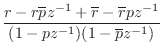
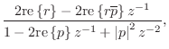
where
When the two poles of a real second-order section are complex, they
form a complex-conjugate pair, i.e., they are located at
![]() in the
in the ![]() plane, where
plane, where ![]() is the modulus of either
pole, and
is the modulus of either
pole, and ![]() is the angle of either pole. In this case, the
``resonance-tuning coefficient'' in Eq.
is the angle of either pole. In this case, the
``resonance-tuning coefficient'' in Eq.![]() (9.3) can be expressed as
(9.3) can be expressed as
Figures 3.25 and 3.26 (p. ![]() ) illustrate filter realizations
consisting of one first-order and two second-order filter sections in
parallel.
) illustrate filter realizations
consisting of one first-order and two second-order filter sections in
parallel.
Next Section:
Implementation of Repeated Poles
Previous Section:
First-Order Complex Resonators


