


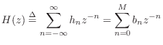
Time Domain Digital Filter Representations
This chapter discusses several time-domain representations for digital filters, including the difference equation, system diagram, and impulse response. Additionally, the convolution representation for LTI filters is derived, and the special case of FIR filters is considered. The transient response, steady-state response, and decay response are examined for FIR and IIR digital filters.
Difference Equation
The difference equation is a formula for computing an output
sample at time ![]() based on past and present input samples and past
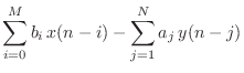
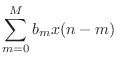
output samples in the time domain.6.1We may write the general, causal, LTI difference equation as follows:
based on past and present input samples and past
output samples in the time domain.6.1We may write the general, causal, LTI difference equation as follows:
where
As a specific example, the difference equation
When the coefficients are real numbers, as in the above example, the filter is said to be real. Otherwise, it may be complex.
Notice that a filter of the form of Eq.![]() (5.1) can use ``past''
output samples (such as
(5.1) can use ``past''
output samples (such as ![]() ) in the calculation of the
``present'' output
) in the calculation of the
``present'' output ![]() . This use of past output samples is called
feedback. Any filter having one or more
feedback paths (
. This use of past output samples is called
feedback. Any filter having one or more
feedback paths (![]() ) is called
recursive. (By
the way, the minus signs for the feedback in Eq.
) is called
recursive. (By
the way, the minus signs for the feedback in Eq.![]() (5.1) will be
explained when we get to transfer functions in §6.1.)
(5.1) will be
explained when we get to transfer functions in §6.1.)
More specifically, the ![]() coefficients are called the
feedforward coefficients and the
coefficients are called the
feedforward coefficients and the ![]() coefficients are called
the feedback coefficients.
coefficients are called
the feedback coefficients.
A filter is said to be recursive if and only if ![]() for
some
for
some ![]() . Recursive filters are also called
infinite-impulse-response (IIR) filters.
When there is no feedback (
. Recursive filters are also called
infinite-impulse-response (IIR) filters.
When there is no feedback (
![]() ), the filter is said
to be a nonrecursive or
finite-impulse-response (FIR) digital filter.
), the filter is said
to be a nonrecursive or
finite-impulse-response (FIR) digital filter.
When used for discrete-time physical modeling, the difference equation may be referred to as an explicit finite difference scheme.6.2
Showing that a recursive filter is LTI (Chapter 4) is easy by considering its impulse-response representation (discussed in §5.6). For example, the recursive filter
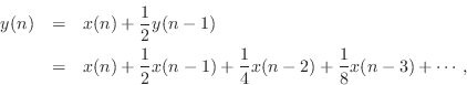
has impulse response
![]() ,
,
![]() . It is now
straightforward to apply the analysis of the previous chapter to find
that time-invariance, superposition, and the scaling property hold.
. It is now
straightforward to apply the analysis of the previous chapter to find
that time-invariance, superposition, and the scaling property hold.
Signal Flow Graph
One possible signal flow graph (or system diagram)
for Eq.![]() (5.1) is given in
Fig.5.1a for the case of
(5.1) is given in
Fig.5.1a for the case of ![]() and
and ![]() .
Hopefully, it is easy to see how this diagram represents the
difference equation (a box labeled ``
.
Hopefully, it is easy to see how this diagram represents the
difference equation (a box labeled ``![]() '' denotes a one-sample
delay in time). The diagram remains true if it is converted to the
frequency domain by replacing all time-domain signals by their
respective z transforms (or Fourier transforms); that is, we may replace
'' denotes a one-sample
delay in time). The diagram remains true if it is converted to the
frequency domain by replacing all time-domain signals by their
respective z transforms (or Fourier transforms); that is, we may replace
![]() by
by ![]() and
and ![]() by
by ![]() .
. ![]() transforms and their usage
will be discussed in Chapter 6.
transforms and their usage
will be discussed in Chapter 6.
 |
Causal Recursive Filters
Equation (5.1) does not cover all LTI filters, for it represents only
causal LTI filters. A filter is said to be
causal when its output does not depend on any ``future'' inputs. (In
more colorful terms, a filter is causal if it does not ``laugh''
before it is ``tickled.'') For example,
![]() is a
non-causal filter because the output anticipates the input one sample
into the future. Restriction to causal filters is quite natural when
the filter operates in real time. Many digital filters, on the other
hand, are implemented on a computer where time is artificially
represented by an array index. Thus, noncausal filters present no
difficulty in such an ``off-line'' situation. It happens that the analysis
for noncausal filters is pretty much the same as that for causal
filters, so we can easily relax this restriction.
is a
non-causal filter because the output anticipates the input one sample
into the future. Restriction to causal filters is quite natural when
the filter operates in real time. Many digital filters, on the other
hand, are implemented on a computer where time is artificially
represented by an array index. Thus, noncausal filters present no
difficulty in such an ``off-line'' situation. It happens that the analysis
for noncausal filters is pretty much the same as that for causal
filters, so we can easily relax this restriction.
Filter Order
The maximum delay, in samples, used in creating each output sample is
called the order
of the filter. In the difference-equation representation, the order is
the larger of ![]() and
and ![]() in Eq.
in Eq.![]() (5.1). For example,
(5.1). For example,
![]() specifies a particular second-order
filter. If
specifies a particular second-order
filter. If ![]() and
and ![]() in
Eq.
in
Eq.![]() (5.1) are constrained to be finite (which is, of course,
necessary in practice), then Eq.
(5.1) are constrained to be finite (which is, of course,
necessary in practice), then Eq.![]() (5.1) represents the class of all
finite-order causal LTI digital filters.
(5.1) represents the class of all
finite-order causal LTI digital filters.
Direct-Form-I Implementation
The difference equation (Eq.![]() (5.1)) is often used as the recipe
for numerical implementation in software or hardware. As such, it
specifies the direct-form I (DF-I) implementation of a digital
filter, one of four direct-form structures to choose from. The DF-I
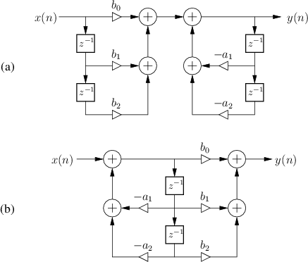
signal flow graph for the second-order case is shown in
Fig.5.1a. The direct-form II structure, another common choice,
is depicted in Fig.5.1b. The other two direct forms are
obtained by transposing direct forms I and II.
Chapter 9 discusses all four direct-form structures.
(5.1)) is often used as the recipe
for numerical implementation in software or hardware. As such, it
specifies the direct-form I (DF-I) implementation of a digital
filter, one of four direct-form structures to choose from. The DF-I
signal flow graph for the second-order case is shown in
Fig.5.1a. The direct-form II structure, another common choice,
is depicted in Fig.5.1b. The other two direct forms are
obtained by transposing direct forms I and II.
Chapter 9 discusses all four direct-form structures.
Impulse-Response Representation
In addition to difference-equation coefficients, any LTI filter may be represented in the time domain by its response to a specific signal called the impulse. This response is called, naturally enough, the impulse response of the filter. Any LTI filter can be implemented by convolving the input signal with the filter impulse response, as we will see.
Definition. The impulse signal is denotedand defined by

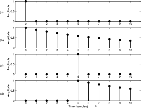
A plot of ![]() is given in Fig.5.2a. In the physical
world, an impulse may be approximated by a swift hammer blow (in the
mechanical case) or balloon pop (acoustic case). We also have a
special notation for the impulse response of a filter:
is given in Fig.5.2a. In the physical
world, an impulse may be approximated by a swift hammer blow (in the
mechanical case) or balloon pop (acoustic case). We also have a
special notation for the impulse response of a filter:
Definition. The impulse response of a filter is the response of the filter to:
We normally require that the impulse response decay to zero over time; otherwise, we say the filter is unstable. The next section formalizes this notion as a definition.
Filter Stability
In this context, we may say that an impulse response ``approaches zero'' by definition if there exists a finite integer
Definition. An LTI filter is said to be stable if the impulse responsegoes to infinity.
Every finite-order nonrecursive filter is stable. Only the feedback
coefficients ![]() in Eq.
in Eq.![]() (5.1) can cause instability. Filter
stability will be discussed further in §8.4 after poles
and zeros have been introduced. Suffice it to say for now that, for
stability, the feedback coefficients must be restricted so that the
feedback gain is less than 1 at every frequency. (We'll learn in
§8.4 that stability is guaranteed when all filter poles
have magnitude less than 1.) In practice, the stability of a
recursive filter is usually checked by computing the filter
reflection coefficients, as described in §8.4.1.
(5.1) can cause instability. Filter
stability will be discussed further in §8.4 after poles
and zeros have been introduced. Suffice it to say for now that, for
stability, the feedback coefficients must be restricted so that the
feedback gain is less than 1 at every frequency. (We'll learn in
§8.4 that stability is guaranteed when all filter poles
have magnitude less than 1.) In practice, the stability of a
recursive filter is usually checked by computing the filter
reflection coefficients, as described in §8.4.1.
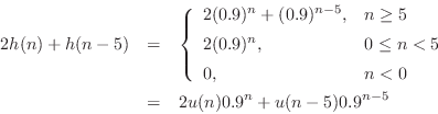
Impulse Response Example
An example impulse response for the first-order recursive filter
is shown in Fig.5.2b. The impulse response is a sampled exponential decay,
![$\displaystyle h(n) = \left\{\begin{array}{ll}
(0.9)^n, & n\geq 0 \\ [5pt]
0, & n<0. \\
\end{array}\right.
$](http://www.dsprelated.com/josimages_new/filters/img550.png)
![$\displaystyle u(n) \isdef \left\{\begin{array}{ll}
1, & n\geq 0 \\ [5pt]
0, & n<0 \\
\end{array}\right.,
$](http://www.dsprelated.com/josimages_new/filters/img551.png)
Implications of Linear-Time-Invariance
Using the basic properties of linearity and time-invariance, we will derive the convolution representation which gives an algorithm for implementing the filter directly in terms of its impulse response. In other words,
 |
The convolution formula plays the role of the difference equation when the impulse response is used in place of the difference-equation coefficients as a filter representation. In fact, we will find that, for FIR filters (nonrecursive, i.e., no feedback), the difference equation and convolution representation are essentially the same thing. For recursive filters, one can think of the convolution representation as the difference equation with all feedback terms ``expanded'' to an infinite number of feedforward terms.
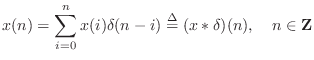
An outline of the derivation of the convolution formula is as follows:
Any signal ![]() may be regarded as a superposition of impulses at
various amplitudes and arrival times, i.e., each sample of
may be regarded as a superposition of impulses at
various amplitudes and arrival times, i.e., each sample of ![]() is
regarded as an impulse with amplitude
is
regarded as an impulse with amplitude ![]() and delay
and delay ![]() . We can
write this mathematically as
. We can
write this mathematically as
![]() . By the
superposition principle for LTI filters, the filter output is simply
the superposition of impulse
responses
. By the
superposition principle for LTI filters, the filter output is simply
the superposition of impulse
responses ![]() , each having a scale factor and time-shift given by
the amplitude and time-shift of the corresponding input impulse.
Thus, the sample
, each having a scale factor and time-shift given by
the amplitude and time-shift of the corresponding input impulse.
Thus, the sample ![]() contributes the signal
contributes the signal
![]() to
the convolution output, and the total output is the sum of such
contributions, by superposition. This is the heart of LTI filtering.
to
the convolution output, and the total output is the sum of such
contributions, by superposition. This is the heart of LTI filtering.
Before proceeding to the general case, let's look at a simple example
with pictures. If an impulse strikes at time ![]() rather than at
time
rather than at
time ![]() , this is represented by writing
, this is represented by writing
![]() . A
picture of this delayed impulse is given in Fig.5.2c. When
. A
picture of this delayed impulse is given in Fig.5.2c. When
![]() is fed to a time-invariant filter, the output will be
the impulse response
is fed to a time-invariant filter, the output will be
the impulse response ![]() delayed by 5 samples, or
delayed by 5 samples, or ![]() . Figure 5.2d shows the response of the example filter of
Eq.
. Figure 5.2d shows the response of the example filter of
Eq.![]() (5.3) to the delayed impulse
(5.3) to the delayed impulse
![]() .
.
In the general case, for time-invariant filters we may write
If two impulses arrive at the filter input, the first at time ![]() ,
say, and the second at time
,
say, and the second at time ![]() , then this input may be expressed
as
, then this input may be expressed
as
![]() . If, in addition, the amplitude of the
first impulse is 2, while the second impulse has an amplitude of 1,
then the input may be written as
. If, in addition, the amplitude of the
first impulse is 2, while the second impulse has an amplitude of 1,
then the input may be written as
![]() . In
this case, using linearity as well as time-invariance, the
response of the general LTI filter to this input may be expressed as
. In
this case, using linearity as well as time-invariance, the
response of the general LTI filter to this input may be expressed as
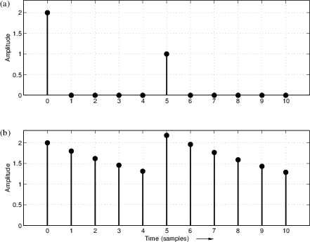
For the example filter of Eq.![]() (5.3), given the input
(5.3), given the input
![]() (pictured in Fig.5.3a),
the output may be computed by scaling, shifting, and adding together
copies of the impulse response
(pictured in Fig.5.3a),
the output may be computed by scaling, shifting, and adding together
copies of the impulse response ![]() . That is, taking the impulse
response in Fig.5.2b, multiplying it by 2, and adding it to the
delayed impulse response in Fig.5.2d, we obtain the output
shown in Fig.5.3b. Thus, a weighted sum of impulses produces
the same weighted sum of impulse responses.
. That is, taking the impulse
response in Fig.5.2b, multiplying it by 2, and adding it to the
delayed impulse response in Fig.5.2d, we obtain the output
shown in Fig.5.3b. Thus, a weighted sum of impulses produces
the same weighted sum of impulse responses.
 |
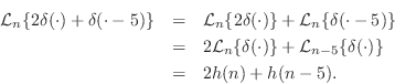
Convolution Representation
We will now derive the convolution representation for LTI filters
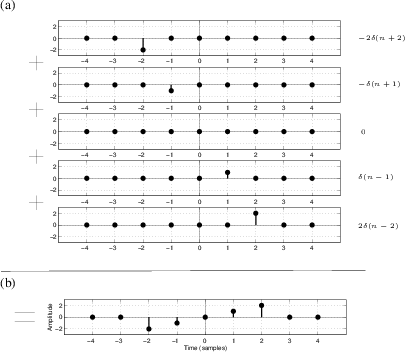
in its full generality. The first step is to express an arbitrary signal
![]() as a linear combination of shifted impulses, i.e.,
as a linear combination of shifted impulses, i.e.,
where ``
If the above equation is not obvious, here is how it is built up
intuitively. Imagine
![]() as a 1 in the midst of an
infinite string of 0s. Now think of
as a 1 in the midst of an
infinite string of 0s. Now think of
![]() as the same
pattern shifted over to the right by
as the same
pattern shifted over to the right by ![]() samples. Next multiply
samples. Next multiply
![]() by
by ![]() , which plucks out the sample
, which plucks out the sample ![]() and surrounds it on both sides by 0's. An example collection of
waveforms
and surrounds it on both sides by 0's. An example collection of
waveforms
![]() for the case
for the case
![]() is shown in
Fig.5.4a. Now, sum over all
is shown in
Fig.5.4a. Now, sum over all ![]() , bringing together the
samples of
, bringing together the
samples of ![]() , to obtain
, to obtain ![]() . Figure 5.4b
shows the result of this addition for the sequences in
Fig.5.4a. Thus, any signal
. Figure 5.4b
shows the result of this addition for the sequences in
Fig.5.4a. Thus, any signal ![]() may be expressed as a
weighted sum of shifted impulses.
may be expressed as a
weighted sum of shifted impulses.
Equation (5.4) expresses a signal as a linear combination (or weighted sum) of impulses. That is, each sample may be viewed as an impulse at some amplitude and time. As we have already seen, each impulse (sample) arriving at the filter's input will cause the filter to produce an impulse response. If another impulse arrives at the filter's input before the first impulse response has died away, then the impulse response for both impulses will superimpose (add together sample by sample). More generally, since the input is a linear combination of impulses, the output is the same linear combination of impulse responses. This is a direct consequence of the superposition principle which holds for any LTI filter.
 |
We repeat this in more precise terms. First linearity is used and then
time-invariance is invoked. Using the form of the general linear
filter in Eq.![]() (4.2), and the definition of linearity,
Eq.
(4.2), and the definition of linearity,
Eq.![]() (4.3) and Eq.
(4.3) and Eq.![]() (4.5),
we can express the output of any linear (and possibly time-varying) filter by
(4.5),
we can express the output of any linear (and possibly time-varying) filter by
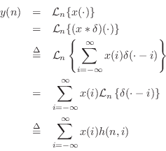
where we have written
![]() to denote the filter
response at time
to denote the filter
response at time ![]() to an impulse which occurred at time
to an impulse which occurred at time ![]() . If we are
to be completely rigorous mathematically, certain ``smoothness''
restrictions must be placed on the linear operator
. If we are
to be completely rigorous mathematically, certain ``smoothness''
restrictions must be placed on the linear operator ![]() in order that
it may be distributed inside the infinite summation [37].
However, practically useful filters of the
form of Eq.
in order that
it may be distributed inside the infinite summation [37].
However, practically useful filters of the
form of Eq.![]() (5.1) satisfy these restrictions. If in addition to
being linear, the filter is time-invariant, then
(5.1) satisfy these restrictions. If in addition to
being linear, the filter is time-invariant, then
![]() ,
which allows us to write
,
which allows us to write
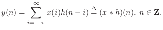
This states that the filter output
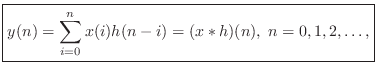
The infinite sum
in Eq.![]() (5.5) can be replaced by more typical practical
limits. By choosing time 0 as the beginning of the signal, we may
define
(5.5) can be replaced by more typical practical
limits. By choosing time 0 as the beginning of the signal, we may
define ![]() to be 0 for
to be 0 for ![]() so that the lower summation limit of
so that the lower summation limit of
![]() can be replaced by 0. Also, if the filter is causal, we
have
can be replaced by 0. Also, if the filter is causal, we
have ![]() for
for ![]() , so the upper summation limit can be
written as
, so the upper summation limit can be
written as ![]() instead of
instead of ![]() . Thus, the
convolution representation of a linear, time-invariant, causal
digital filter is given by
. Thus, the
convolution representation of a linear, time-invariant, causal
digital filter is given by
Since the above equation is a convolution, and since convolution is
commutative (i.e.,
![]() [84]), we
can rewrite it as
[84]), we
can rewrite it as
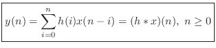
Convolution Representation Summary
We have shown that the output ![]() of any LTI filter may be calculated
by convolving the input
of any LTI filter may be calculated
by convolving the input ![]() with the impulse response
with the impulse response ![]() . It is
instructive to compare this method of filter implementation to the use
of difference equations, Eq.
. It is
instructive to compare this method of filter implementation to the use
of difference equations, Eq.![]() (5.1). If there is no feedback (no
(5.1). If there is no feedback (no
![]() coefficients in Eq.
coefficients in Eq.![]() (5.1)), then the difference equation and
the convolution formula are essentially identical, as shown in
the next section.
For recursive filters, we can convert the difference equation into a
convolution by calculating the filter impulse response. However, this
can be rather tedious, since with nonzero feedback coefficients the
impulse response generally lasts forever. Of course, for stable
filters the response is infinite only in theory; in practice, one may
truncate the response after an appropriate length of time, such as
after it falls below the quantization noise level due to round-off
error.
(5.1)), then the difference equation and
the convolution formula are essentially identical, as shown in
the next section.
For recursive filters, we can convert the difference equation into a
convolution by calculating the filter impulse response. However, this
can be rather tedious, since with nonzero feedback coefficients the
impulse response generally lasts forever. Of course, for stable
filters the response is infinite only in theory; in practice, one may
truncate the response after an appropriate length of time, such as
after it falls below the quantization noise level due to round-off
error.
Finite Impulse Response Digital Filters
In §5.1 we defined the general difference equation for IIR filters, and a couple of second-order examples were diagrammed in Fig.5.1. In this section, we take a more detailed look at the special case of Finite Impulse Response (FIR) digital filters. In addition to introducing various terminology and practical considerations associated with FIR filters, we'll look at a preview of transfer-function analysis (Chapter 6) for this simple special case.
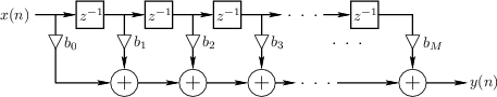 |
Figure 5.5 gives the signal flow graph for a general causal FIR filter Such a filter is also called a transversal filter, or a tapped delay line. The implementation shown is classified as a direct-form implementation.
FIR impulse response
The impulse response ![]() is obtained at the output when the
input signal is the impulse signal
is obtained at the output when the
input signal is the impulse signal
![]() (§5.6). If the
(§5.6). If the ![]() th tap is denoted
th tap is denoted ![]() , then it is
obvious from Fig.5.5 that the impulse response signal is
given by
, then it is
obvious from Fig.5.5 that the impulse response signal is
given by
![$\displaystyle h(n)\isdef \left\{\begin{array}{ll} 0, & n<0 \\ [5pt] b_n, & 0\leq n\leq M \\ [5pt] 0, & n> M \\ \end{array} \right. \protect$](http://www.dsprelated.com/josimages_new/filters/img596.png)
In other words, the impulse response simply consists of the tap coefficients, prepended and appended by zeros.
Convolution Representation of FIR Filters
Notice that the output of the ![]() th delay element in Fig.5.5 is
th delay element in Fig.5.5 is
![]() ,
,
![]() , where
, where ![]() is the input signal
amplitude at time
is the input signal
amplitude at time ![]() . The output signal
. The output signal ![]() is therefore
is therefore
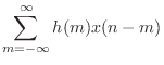
where we have used the convolution operator ``
The ``Finite'' in FIR
From Eq.![]() (5.7), we can see that the impulse response becomes zero
after time
(5.7), we can see that the impulse response becomes zero
after time ![]() . Therefore, a tapped delay line (Fig.5.5) can
only implement finite-duration impulse responses in the sense
that the non-zero portion of the impulse response must be finite.
This is what is meant by the term finite impulse response
(FIR). We may say that the impulse response has finite support
[52].
. Therefore, a tapped delay line (Fig.5.5) can
only implement finite-duration impulse responses in the sense
that the non-zero portion of the impulse response must be finite.
This is what is meant by the term finite impulse response
(FIR). We may say that the impulse response has finite support
[52].
Causal FIR Filters
From Eq.![]() (5.6), we see also that the impulse response
(5.6), we see also that the impulse response ![]() is
always zero for
is
always zero for ![]() . Recall from §5.3 that any LTI
filter having a zero impulse response prior to time 0 is said to be
causal. Thus, a tapped delay line such as that depicted in
Fig.5.5 can only implement causal FIR filters. In software,
on the other hand, we may easily implement non-causal FIR filters as
well, based simply on the definition of convolution.
. Recall from §5.3 that any LTI
filter having a zero impulse response prior to time 0 is said to be
causal. Thus, a tapped delay line such as that depicted in
Fig.5.5 can only implement causal FIR filters. In software,
on the other hand, we may easily implement non-causal FIR filters as
well, based simply on the definition of convolution.
FIR Transfer Function
The transfer function of an FIR filter is given by the z transform of
its impulse response. This is true for any LTI filter, as discussed
in Chapter 6. For FIR filters in particular, we have, from
Eq.![]() (5.6),
(5.6),
Thus, the transfer function of every length
FIR Order
The order of a filter is defined as the order of its transfer
function, as discussed in Chapter 6. For FIR filters, this is just
the order of the transfer-function polynomial. Thus, from
Equation (5.8), the order of the general, causal, length ![]() FIR
filter is
FIR
filter is ![]() (provided
(provided ![]() ).
).
Note from Fig.5.5 that the order ![]() is also the total number
of delay elements in the filter. This is typical of practical
digital filter implementations. When the number of delay elements in
the implementation (Fig.5.5) is equal to the filter order, the
filter implementation is said to be canonical with respect to
delay. It is not possible to implement a given transfer function in
fewer delays than the transfer function order, but it is possible (and
sometimes even desirable) to have extra delays.
is also the total number
of delay elements in the filter. This is typical of practical
digital filter implementations. When the number of delay elements in
the implementation (Fig.5.5) is equal to the filter order, the
filter implementation is said to be canonical with respect to
delay. It is not possible to implement a given transfer function in
fewer delays than the transfer function order, but it is possible (and
sometimes even desirable) to have extra delays.
FIR Software Implementations
In matlab, an efficient FIR filter is implemented by calling
outputsignal = filter(B,1,inputsignal);
where
Figure 5.6 lists a second-order FIR filter implementation in the C programming language.
typedef double *pp; // pointer to array of length NTICK typedef double word; // signal and coefficient data type typedef struct _fir3Vars { pp outputAout; pp inputAinp; word b0; word b1; word b2; word s1; word s2; } fir3Vars; void fir3(fir3Vars *a) { int i; word input; for (i=0; i<NTICK; i++) { input = a->inputAinp[i]; a->outputAout[i] = a->b0 * input + a->b1 * a->s1 + a->b2 * a->s2; a->s2 = a->s1; a->s1 = input; } } |
Transient Response, Steady State, and Decay

Input
Signal 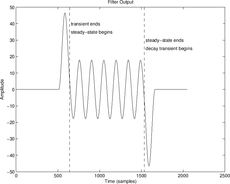
Filter Output Signal
|
The terms transient response and steady state response
arise naturally in the context of sinewave analysis (e.g.,
§2.2). When the input sinewave is switched on, the filter
takes a while to ``settle down'' to a perfect sinewave at the same
frequency, as illustrated in Fig.5.12. The filter response during
this ``settling'' period is called the transient response of
the filter. The response of the filter after the transient
response, provided the filter is linear and time-invariant, is called
the steady-state response, and it consists of a pure sinewave
at the same frequency as the input sinewave, but with amplitude and
phase determined by the filter's frequency response at that
frequency. In other words, the steady-state response begins when the
LTI filter is fully ``warmed up'' by the input signal. More
precisely, the filter output is the same as if the input signal had
been applied since time minus infinity. Length ![]() FIR filters
only ``remember''
FIR filters
only ``remember'' ![]() samples into the past.
Thus, for length
samples into the past.
Thus, for length ![]() FIR filters, the duration of the transient response is
FIR filters, the duration of the transient response is
![]() samples.
samples.
To show this, (it may help to refer to the general FIR filter
implementation in Fig.5.5), consider that a length ![]() (zero-order) FIR filter (a simple gain), has no state memory at all,
and thus it is in ``steady state'' immediately when the input sinewave
is switched on. A length
(zero-order) FIR filter (a simple gain), has no state memory at all,
and thus it is in ``steady state'' immediately when the input sinewave
is switched on. A length ![]() FIR filter, on the other hand, reaches
steady state one sample after the input sinewave is switched on,
because it has one sample of delay. At the switch-on time instant,
the length 2 FIR filter has a single sample of state that is still
zero (instead of its steady-state value which is the previous input
sinewave sample).
FIR filter, on the other hand, reaches
steady state one sample after the input sinewave is switched on,
because it has one sample of delay. At the switch-on time instant,
the length 2 FIR filter has a single sample of state that is still
zero (instead of its steady-state value which is the previous input
sinewave sample).
In general, a length ![]() FIR filter is fully ``warmed up'' after
FIR filter is fully ``warmed up'' after ![]() samples of input; that is, for an input starting at time
samples of input; that is, for an input starting at time ![]() , by
time
, by
time ![]() , all internal state delays of the filter contain delayed
input samples instead of their initial zeros. When the input signal is
a unit step
, all internal state delays of the filter contain delayed
input samples instead of their initial zeros. When the input signal is
a unit step ![]() times a sinusoid (or, by superposition, any linear
combination of sinusoids), we may say that the filter output reaches
steady state at time
times a sinusoid (or, by superposition, any linear
combination of sinusoids), we may say that the filter output reaches
steady state at time ![]() .
.
FIR Example
An example sinewave input signal is shown in Fig.5.12, and
the output of a length ![]() FIR ``running sum'' filter is shown in
Fig.5.12. These signals were computed by the following matlab
code:
FIR ``running sum'' filter is shown in
Fig.5.12. These signals were computed by the following matlab
code:
  Nx = 1024; % input signal length (nonzero portion)
  Nh = 128;  % FIR filter length
  A = 1; B = ones(1,Nh); % FIR "running sum" filter
  n = 0:Nx-1;
  x = sin(n*2*pi*7/Nx);  % input sinusoid - zero-pad it:
  zp=zeros(1,Nx/2); xzp=[zp,x,zp]; nzp=[0:length(xzp)-1];
  y = filter(B,A,xzp);   % filtered output signal
We know that the transient response must end
Since the coefficients of an FIR filter are also its nonzero impulse response samples, we can say that the duration of the transient response equals the length of the impulse response minus one.
For Infinite Impulse Response (IIR) filters, such as the recursive
comb filter analyzed in Chapter 3, the transient response
decays exponentially. This means it is never really completely
finished. In other terms, since its impulse response is infinitely
long, so is its transient response, in principle. However, in
practice, we treat it as finished for all practical purposes after
several time constants of decay. For example, seven time-constants of
decay correspond to more than 60 dB of decay, and is a common cut-off
used for audio purposes. Therefore, we can adopt ![]() as the
definition of decay time (or ``ring time'') for typical
audio filters. See [84]6.5 for a detailed derivation
of
as the
definition of decay time (or ``ring time'') for typical
audio filters. See [84]6.5 for a detailed derivation
of ![]() and related topics. In summary, we can say that the
transient response of an audio filter is over after
and related topics. In summary, we can say that the
transient response of an audio filter is over after ![]() seconds,
where
seconds,
where ![]() is the time it takes the filter impulse response to
decay by
is the time it takes the filter impulse response to
decay by ![]() dB.
dB.
IIR Example
Figure 5.8 plots an IIR filter example for the filter
      Nh = 300; % APPROXIMATE filter length (visually in plot)
      B = 1; A = [1 -0.99]; % One-pole recursive example
      ...       % otherwise as above for the FIR example
The decay time for this recursive filter was arbitrarily marked at 300
samples (about three time-constants of decay).

Input
Signal 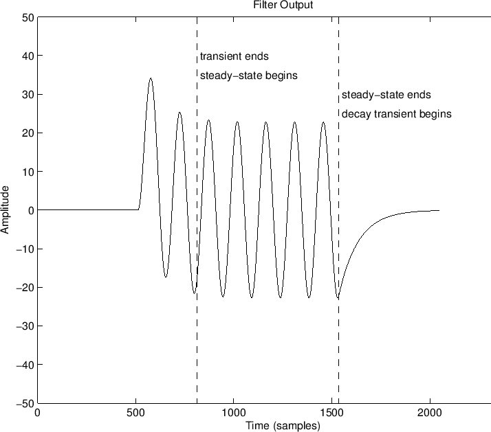
Filter Output Signal
|
Transient and Steady-State Signals
Loosely speaking, any sudden change in a signal is regarded as a transient, and transients in an input signal disturb the steady-state operation of a filter, resulting in a transient response at the filter output. This leads us to ask how do we define ``transient'' in a precise way? This turns out to be difficult in practice.
A mathematically convenient definition is as follows: A signal is said to contain a transient whenever its Fourier expansion [84] requires an infinite number of sinusoids. Conversely, any signal expressible as a finite number of sinusoids can be defined as a steady-state signal. Thus, waveform discontinuities are transients, as are discontinuities in the waveform slope, curvature, etc. Any fixed sum of sinusoids, on the other hand, is a steady-state signal.
In practical audio signal processing, defining transients is more difficult. In particular, since hearing is bandlimited, all audible signals are technically steady-state signals under the above definition. One way to pose the question is to ask which sounds should be ``stretched'' and which should be translated in time when a signal is ``slowed down''? In the case of speech, for example, short consonants would be considered transients, while vowels and sibilants such as ``ssss'' would be considered steady-state signals. Percussion hits are generally considered transients, as are the ``attacks'' of plucked and struck strings (such as piano). More generally, almost any ``attack'' is considered a transient, but a slow fade-in of a string section, e.g., might not be. In sum, musical discrimination between ``transient'' and ``steady state'' signals depends on our perception, and on our learned classifications of sounds. However, to first order, transient sounds can be defined practically as sudden ``wideband events'' in an otherwise steady-state signal. This is at least similar in spirit to the mathematical definition given above.
In summary, a filter transient response is caused by suddenly switching on a filter input signal, or otherwise disturbing a steady-state input signal away from its steady-state form. After the transient response has died out, we see the steady-state response, provided that the input signal itself is a steady-state signal (a fixed linear combination of sinusoids) and given that the filter is LTI.
Decay Response, Initial Conditions Response
If a filter is in steady state and we switch off the input signal, we see its decay response. This response is identical (but for a time shift) to the filter's response to initial conditions. In other words, when the input signal is switched off (becomes zero), the future output signal is computed entirely from the filter's internal state, because the input signal remains zero.
Complete Response
In general, the so-called complete response of a linear, time-invariant filter is given by the superposition of its
``Zero-state response'' simply means the response of the filter to an input signal when the initial state of the filter (all its memory cells) are zeroed to begin with. The initial-condition response is of course the response of the filter to its own initial state, with the input signal being zero. This clean superposition of the zero-state and initial-condition responses only holds in general for linear filters. In §G.3, this superposition will be considered for state-space filter representations.
Summary and Conclusions
This concludes the discussion of time-domain filter descriptions, including difference equations, signal flow graphs, and impulse-response representations. More time-domain forms (alternative digital filter implementations) will be described in Chapter 9. A tour of elementary digital filter sections used often in audio applications is presented in Appendix B. Beyond that, some matrix-based representations are included in Appendix F, and the state-space formulation is discussed in Appendix G.
Time-domain forms are typically used to implement recursive filters in software or hardware, and they generalize readily to nonlinear and/or time-varying cases. For an understanding of the effects of an LTI filter on a sound, however, it is usually more appropriate to consider a frequency-domain picture, to which we now turn in the next chapter.
Time Domain Representation Problems
See http://ccrma.stanford.edu/~jos/filtersp/Time_Domain_Representation_Problems.html.
Next Section:
Transfer Function Analysis
Previous Section:
Linear Time-Invariant Digital Filters


