


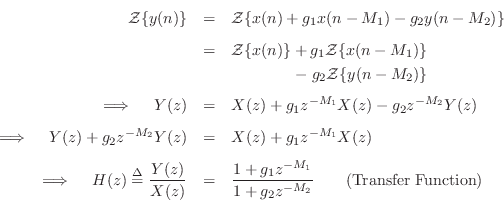
Transfer Function
As we cover in Chapter 6, the transfer function of a digital filter
is defined as
![]() where
where ![]() is the z transform of the input
signal
is the z transform of the input
signal ![]() , and
, and ![]() is the z transform of the output signal
is the z transform of the output signal ![]() . We
may find
. We
may find ![]() from Eq.
from Eq.![]() (3.1) by taking the z transform of both sides
and solving for
(3.1) by taking the z transform of both sides
and solving for ![]() :
:
Some principles of this analysis are as follows:
- The z transform
 is a linear operator which means, by definition,

-
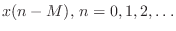
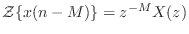 . That is, the z transform of a signal
  delayed by
  samples,
 , is
, is
 . This is the shift theorem for z transforms, which can
be immediately derived from the definition of the z transform, as shown in
§6.3.
. This is the shift theorem for z transforms, which can
be immediately derived from the definition of the z transform, as shown in
§6.3.
In matlab, difference-equation coefficients are specified as
transfer-function coefficients (vectors B and A in Fig.3.9).
This is why a minus sign is needed in Eq.![]() (3.3).
(3.3).
Ok, so finding the transfer function is not too much work. Now, what
can we do with it? There are two main avenues of analysis from here:
(1) finding the frequency response by setting
![]() , and
(2) factoring the transfer function to find the poles and
zeros of the filter. One also uses the transfer function to generate
different implementation forms such as cascade or parallel
combinations of smaller filters to achieve the same overall filter.
The following sections will illustrate these uses of the transfer
function on the example filter of this chapter.
, and
(2) factoring the transfer function to find the poles and
zeros of the filter. One also uses the transfer function to generate
different implementation forms such as cascade or parallel
combinations of smaller filters to achieve the same overall filter.
The following sections will illustrate these uses of the transfer
function on the example filter of this chapter.
Next Section:
Frequency Response
Previous Section:
Impulse Response


