


Transient Response, Steady State, and Decay

Input
Signal 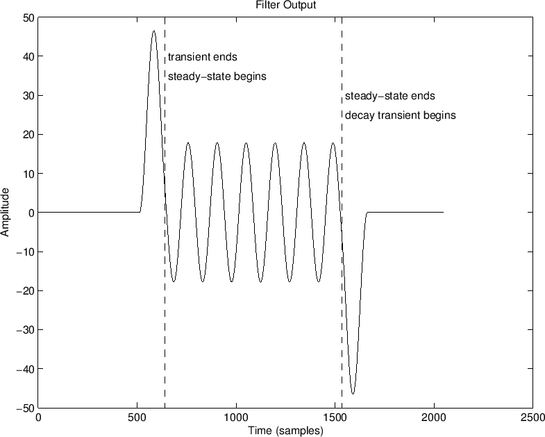
Filter Output Signal
|
The terms transient response and steady state response
arise naturally in the context of sinewave analysis (e.g.,
§2.2). When the input sinewave is switched on, the filter
takes a while to ``settle down'' to a perfect sinewave at the same
frequency, as illustrated in Fig.5.12. The filter response during
this ``settling'' period is called the transient response of
the filter. The response of the filter after the transient
response, provided the filter is linear and time-invariant, is called
the steady-state response, and it consists of a pure sinewave
at the same frequency as the input sinewave, but with amplitude and
phase determined by the filter's frequency response at that
frequency. In other words, the steady-state response begins when the
LTI filter is fully ``warmed up'' by the input signal. More
precisely, the filter output is the same as if the input signal had
been applied since time minus infinity. Length ![]() FIR filters
only ``remember''
FIR filters
only ``remember'' ![]() samples into the past.
Thus, for length
samples into the past.
Thus, for length ![]() FIR filters, the duration of the transient response is
FIR filters, the duration of the transient response is
![]() samples.
samples.
To show this, (it may help to refer to the general FIR filter
implementation in Fig.5.5), consider that a length ![]() (zero-order) FIR filter (a simple gain), has no state memory at all,
and thus it is in ``steady state'' immediately when the input sinewave
is switched on. A length
(zero-order) FIR filter (a simple gain), has no state memory at all,
and thus it is in ``steady state'' immediately when the input sinewave
is switched on. A length ![]() FIR filter, on the other hand, reaches
steady state one sample after the input sinewave is switched on,
because it has one sample of delay. At the switch-on time instant,
the length 2 FIR filter has a single sample of state that is still
zero (instead of its steady-state value which is the previous input
sinewave sample).
FIR filter, on the other hand, reaches
steady state one sample after the input sinewave is switched on,
because it has one sample of delay. At the switch-on time instant,
the length 2 FIR filter has a single sample of state that is still
zero (instead of its steady-state value which is the previous input
sinewave sample).
In general, a length ![]() FIR filter is fully ``warmed up'' after
FIR filter is fully ``warmed up'' after ![]() samples of input; that is, for an input starting at time
samples of input; that is, for an input starting at time ![]() , by
time
, by
time ![]() , all internal state delays of the filter contain delayed
input samples instead of their initial zeros. When the input signal is
a unit step
, all internal state delays of the filter contain delayed
input samples instead of their initial zeros. When the input signal is
a unit step ![]() times a sinusoid (or, by superposition, any linear
combination of sinusoids), we may say that the filter output reaches
steady state at time
times a sinusoid (or, by superposition, any linear
combination of sinusoids), we may say that the filter output reaches
steady state at time ![]() .
.
FIR Example
An example sinewave input signal is shown in Fig.5.12, and
the output of a length ![]() FIR ``running sum'' filter is shown in
Fig.5.12. These signals were computed by the following matlab
code:
FIR ``running sum'' filter is shown in
Fig.5.12. These signals were computed by the following matlab
code:
  Nx = 1024; % input signal length (nonzero portion)
  Nh = 128;  % FIR filter length
  A = 1; B = ones(1,Nh); % FIR "running sum" filter
  n = 0:Nx-1;
  x = sin(n*2*pi*7/Nx);  % input sinusoid - zero-pad it:
  zp=zeros(1,Nx/2); xzp=[zp,x,zp]; nzp=[0:length(xzp)-1];
  y = filter(B,A,xzp);   % filtered output signal
We know that the transient response must end
Since the coefficients of an FIR filter are also its nonzero impulse response samples, we can say that the duration of the transient response equals the length of the impulse response minus one.
For Infinite Impulse Response (IIR) filters, such as the recursive
comb filter analyzed in Chapter 3, the transient response
decays exponentially. This means it is never really completely
finished. In other terms, since its impulse response is infinitely
long, so is its transient response, in principle. However, in
practice, we treat it as finished for all practical purposes after
several time constants of decay. For example, seven time-constants of
decay correspond to more than 60 dB of decay, and is a common cut-off
used for audio purposes. Therefore, we can adopt ![]() as the
definition of decay time (or ``ring time'') for typical
audio filters. See [84]6.5 for a detailed derivation
of
as the
definition of decay time (or ``ring time'') for typical
audio filters. See [84]6.5 for a detailed derivation
of ![]() and related topics. In summary, we can say that the
transient response of an audio filter is over after
and related topics. In summary, we can say that the
transient response of an audio filter is over after ![]() seconds,
where
seconds,
where ![]() is the time it takes the filter impulse response to
decay by
is the time it takes the filter impulse response to
decay by ![]() dB.
dB.
IIR Example
Figure 5.8 plots an IIR filter example for the filter
      Nh = 300; % APPROXIMATE filter length (visually in plot)
      B = 1; A = [1 -0.99]; % One-pole recursive example
      ...       % otherwise as above for the FIR example
The decay time for this recursive filter was arbitrarily marked at 300
samples (about three time-constants of decay).

Input
Signal 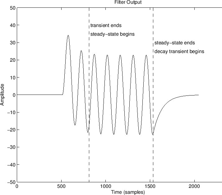
Filter Output Signal
|
Transient and Steady-State Signals
Loosely speaking, any sudden change in a signal is regarded as a transient, and transients in an input signal disturb the steady-state operation of a filter, resulting in a transient response at the filter output. This leads us to ask how do we define ``transient'' in a precise way? This turns out to be difficult in practice.
A mathematically convenient definition is as follows: A signal is said to contain a transient whenever its Fourier expansion [84] requires an infinite number of sinusoids. Conversely, any signal expressible as a finite number of sinusoids can be defined as a steady-state signal. Thus, waveform discontinuities are transients, as are discontinuities in the waveform slope, curvature, etc. Any fixed sum of sinusoids, on the other hand, is a steady-state signal.
In practical audio signal processing, defining transients is more difficult. In particular, since hearing is bandlimited, all audible signals are technically steady-state signals under the above definition. One way to pose the question is to ask which sounds should be ``stretched'' and which should be translated in time when a signal is ``slowed down''? In the case of speech, for example, short consonants would be considered transients, while vowels and sibilants such as ``ssss'' would be considered steady-state signals. Percussion hits are generally considered transients, as are the ``attacks'' of plucked and struck strings (such as piano). More generally, almost any ``attack'' is considered a transient, but a slow fade-in of a string section, e.g., might not be. In sum, musical discrimination between ``transient'' and ``steady state'' signals depends on our perception, and on our learned classifications of sounds. However, to first order, transient sounds can be defined practically as sudden ``wideband events'' in an otherwise steady-state signal. This is at least similar in spirit to the mathematical definition given above.
In summary, a filter transient response is caused by suddenly switching on a filter input signal, or otherwise disturbing a steady-state input signal away from its steady-state form. After the transient response has died out, we see the steady-state response, provided that the input signal itself is a steady-state signal (a fixed linear combination of sinusoids) and given that the filter is LTI.
Decay Response, Initial Conditions Response
If a filter is in steady state and we switch off the input signal, we see its decay response. This response is identical (but for a time shift) to the filter's response to initial conditions. In other words, when the input signal is switched off (becomes zero), the future output signal is computed entirely from the filter's internal state, because the input signal remains zero.
Complete Response
In general, the so-called complete response of a linear, time-invariant filter is given by the superposition of its
``Zero-state response'' simply means the response of the filter to an input signal when the initial state of the filter (all its memory cells) are zeroed to begin with. The initial-condition response is of course the response of the filter to its own initial state, with the input signal being zero. This clean superposition of the zero-state and initial-condition responses only holds in general for linear filters. In §G.3, this superposition will be considered for state-space filter representations.
Next Section:
Summary and Conclusions
Previous Section:
Finite Impulse Response Digital Filters


