


Introduction to the DFT
This chapter introduces the Discrete Fourier Transform (DFT) and
points out the mathematical elements that will be explicated in this
book. To find motivation for a detailed study of the DFT, the reader
might first peruse Chapter 8 to get a feeling for some of the many
practical applications of the DFT. (See also the preface on page
![]() .)
.)
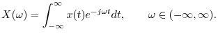
Before we get started on the DFT, let's look for a moment at the
Fourier transform (FT) and explain why we are not talking about
it instead. The Fourier transform of a continuous-time signal ![]() may be defined as
may be defined as
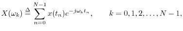
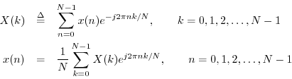
DFT Definition
The Discrete Fourier Transform (DFT) of a signal ![]() may be defined by
may be defined by
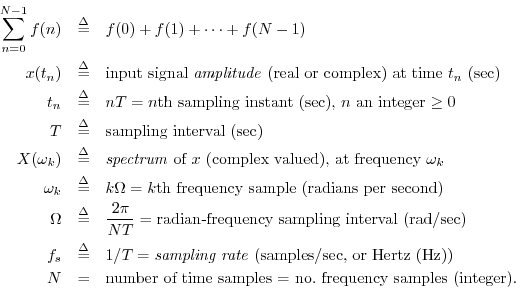
The sampling interval ![]() is also called the sampling period.
For a tutorial on sampling continuous-time signals to obtain
non-aliased discrete-time signals, see Appendix D.
is also called the sampling period.
For a tutorial on sampling continuous-time signals to obtain
non-aliased discrete-time signals, see Appendix D.
When all ![]() signal samples
signal samples ![]() are real, we say
are real, we say
![]() .
If they may be complex, we write
.
If they may be complex, we write
![]() . Finally,
. Finally,
![]() means
means ![]() is any integer.
is any integer.
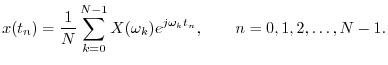
Inverse DFT
The inverse DFT (the IDFT) is given by
Mathematics of the DFT
In the signal processing literature, it is common to write the DFT
and its inverse in the
more pure form below, obtained by setting ![]() in the previous definition:
in the previous definition:
where ![]() denotes the input signal at time (sample)
denotes the input signal at time (sample) ![]() , and
, and ![]() denotes the
denotes the ![]() th spectral sample. This form is the simplest
mathematically, while the previous form is easier to interpret
physically.
th spectral sample. This form is the simplest
mathematically, while the previous form is easier to interpret
physically.
There are two remaining symbols in the DFT we have not yet defined:
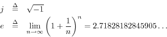
The first,
![]() , is the basis for complex
numbers.1.1 As a result, complex numbers will be the
first topic we cover in this book (but only to the extent needed
to understand the DFT).
, is the basis for complex
numbers.1.1 As a result, complex numbers will be the
first topic we cover in this book (but only to the extent needed
to understand the DFT).
The second,
![]() , is a (transcendental) real number
defined by the above limit. We will derive
, is a (transcendental) real number
defined by the above limit. We will derive ![]() and talk about why it
comes up in Chapter 3.
and talk about why it
comes up in Chapter 3.
Note that not only do we have complex numbers to contend with, but we have them appearing in exponents, as in
With ![]() ,
, ![]() , and imaginary exponents understood, we can go on to prove
Euler's Identity:
, and imaginary exponents understood, we can go on to prove
Euler's Identity:
Finally, we need to understand what the summation over ![]() is doing in
the definition of the DFT. We'll learn that it should be seen as the
computation of the inner product of the signals
is doing in
the definition of the DFT. We'll learn that it should be seen as the
computation of the inner product of the signals ![]() and
and ![]() defined above, so that we may write the DFT, using inner-product
notation, as
defined above, so that we may write the DFT, using inner-product
notation, as

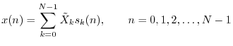
After the foregoing, the inverse DFT can be understood as the
sum of projections of ![]() onto
onto
![]() ; i.e.,
we'll show
; i.e.,
we'll show

Having completely understood the DFT and its inverse mathematically, we go on to proving various Fourier Theorems, such as the ``shift theorem,'' the ``convolution theorem,'' and ``Parseval's theorem.'' The Fourier theorems provide a basic thinking vocabulary for working with signals in the time and frequency domains. They can be used to answer questions such as
``What happens in the frequency domain if I do [operation x] in the time domain?''Usually a frequency-domain understanding comes closest to a perceptual understanding of audio processing.
Finally, we will study a variety of practical spectrum analysis examples, using primarily the matlab programming language [67] to analyze and display signals and their spectra.
DFT Math Outline
In summary, understanding the DFT takes us through the following topics:
- Complex numbers
- Complex exponents
- Why
 ?
?
- Euler's identity
- Projecting signals onto signals via the inner product
- The DFT as the coefficient of projection of a signal
 onto a sinusoid
- The IDFT as a sum of projections onto sinusoids
- Various Fourier theorems
- Elementary time-frequency pairs
- Practical spectrum analysis in matlab
We will additionally discuss various practical aspects of working with signals and spectra.
Next Section:
Complex Numbers
Previous Section:
Preface


