


Matched Filtering
The cross-correlation function is used extensively in pattern
recognition and signal detection. We know from Chapter 5
that projecting one signal onto another is a means of measuring how
much of the second signal is present in the first. This can be used
to ``detect'' the presence of known signals as components of more
complicated signals. As a simple example, suppose we record ![]() which we think consists of a signal
which we think consists of a signal ![]() that we are looking for
plus some additive measurement noise
that we are looking for
plus some additive measurement noise ![]() . That is, we assume the
signal model
. That is, we assume the
signal model
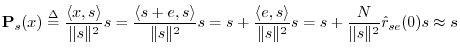
![]() . Then the projection of
. Then the projection of ![]() onto
onto ![]() is
(recalling §5.9.9)
is
(recalling §5.9.9)
In the same way that FFT convolution is faster than direct convolution (see Table 7.1), cross-correlation and matched filtering are generally carried out most efficiently using an FFT algorithm (Appendix A).
Next Section:
FIR System Identification
Previous Section:
Autocorrelation


