


Signal Operators
It will be convenient in the Fourier theorems of §7.4 to make use of the following signal operator definitions.
Operator Notation
In this book, an operator is defined as a
signal-valued function of a signal. Thus, for the space
of length ![]() complex sequences, an operator
complex sequences, an operator
![]() is a mapping
from
is a mapping
from ![]() to
to ![]() :
:
Note that operator notation is not standard in the field of
digital signal processing. It can be regarded as being influenced by
the field of computer science. In the Fourier theorems below, both
operator and conventional signal-processing notations are provided. In the
author's opinion, operator notation is consistently clearer, allowing
powerful expressions to be written naturally in one line (e.g., see
Eq.![]() (7.8)), and it is much closer to how things look in
a readable computer program (such as in the matlab language).
(7.8)), and it is much closer to how things look in
a readable computer program (such as in the matlab language).
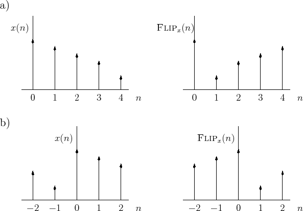
Flip Operator
We define the flip operator by
for all sample indices
Shift Operator
The shift operator is defined by
![\includegraphics[width=\twidth]{eps/shift}](http://www.dsprelated.com/josimages_new/mdft/img1153.png) |
Figure 7.2 illustrates successive one-sample delays of a periodic signal
having first period given by
![]() .
.
Examples
-
![$ \hbox{\sc Shift}_1([1,0,0,0]) = [0,1,0,0]\;$](http://www.dsprelated.com/josimages_new/mdft/img1154.png) (an impulse delayed one sample).
(an impulse delayed one sample).
-
![$ \hbox{\sc Shift}_1([1,2,3,4]) = [4,1,2,3]\;$](http://www.dsprelated.com/josimages_new/mdft/img1155.png) (a circular shift example).
(a circular shift example).
-
![$ \hbox{\sc Shift}_{-2}([1,0,0,0]) = [0,0,1,0]\;$](http://www.dsprelated.com/josimages_new/mdft/img1156.png) (another circular shift example).
(another circular shift example).
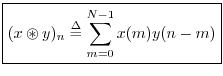
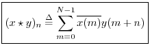
Convolution
The convolution of two signals ![]() and
and ![]() in
in ![]() may be
denoted ``
may be
denoted ``
![]() '' and defined by
'' and defined by
Cyclic convolution can be expressed in terms of previously defined operators as
Commutativity of Convolution
Convolution (cyclic or acyclic) is commutative, i.e.,
Proof:
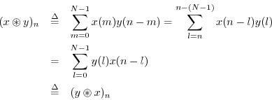
In the first step we made the change of summation variable
![]() , and in the second step, we made use of the fact
that any sum over all
, and in the second step, we made use of the fact
that any sum over all ![]() terms is equivalent to a sum from 0 to
terms is equivalent to a sum from 0 to
![]() .
.
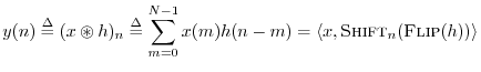
Convolution as a Filtering Operation
In a convolution of two signals
![]() , where both
, where both ![]() and
and ![]() are signals of length
are signals of length ![]() (real or complex), we may interpret either
(real or complex), we may interpret either
![]() or
or ![]() as a filter that operates on the other signal
which is in turn interpreted as the filter's ``input signal''.7.5 Let
as a filter that operates on the other signal
which is in turn interpreted as the filter's ``input signal''.7.5 Let
![]() denote a length
denote a length ![]() signal that is interpreted
as a filter. Then given any input signal
signal that is interpreted
as a filter. Then given any input signal
![]() , the filter output
signal
, the filter output
signal
![]() may be defined as the cyclic convolution of
may be defined as the cyclic convolution of
![]() and
and ![]() :
:
![$\displaystyle \delta(n) = \left\{\begin{array}{ll}
1, & n=0\;\mbox{(mod $N$)} \\ [5pt]
0, & n\ne 0\;\mbox{(mod $N$)}. \\
\end{array} \right.
$](http://www.dsprelated.com/josimages_new/mdft/img1170.png)
![$\displaystyle \delta(n) \isdef \left\{\begin{array}{ll}
1, & n=0 \\ [5pt]
0, & n\ne 0 \\
\end{array} \right.
$](http://www.dsprelated.com/josimages_new/mdft/img1172.png)
As discussed below (§7.2.7), one may embed acyclic convolution within a larger cyclic convolution. In this way, real-world systems may be simulated using fast DFT convolutions (see Appendix A for more on fast convolution algorithms).
Note that only linear, time-invariant (LTI) filters can be completely represented by their impulse response (the filter output in response to an impulse at time 0). The convolution representation of LTI digital filters is fully discussed in Book II [68] of the music signal processing book series (in which this is Book I).
Convolution Example 1: Smoothing a Rectangular Pulse
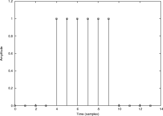
Filter
input signal 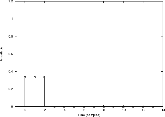
Filter impulse response 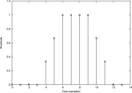
Filter output signal |
Figure 7.3 illustrates convolution of
![$\displaystyle h = \left[\frac{1}{3},\frac{1}{3},\frac{1}{3},0,0,0,0,0,0,0,0,0,0,0\right]
$](http://www.dsprelated.com/josimages_new/mdft/img1177.png)
![$\displaystyle y = x\circledast h = \left[0,0,0,0,\frac{1}{3},\frac{2}{3},1,1,1,1,\frac{2}{3},\frac{1}{3},0,0\right] \protect$](http://www.dsprelated.com/josimages_new/mdft/img1178.png)
as graphed in Fig.7.3(c). In this case,
![$\displaystyle h=\left[\frac{1}{3},\frac{1}{3},0,0,0,0,0,0,0,0,0,0,\frac{1}{3}\right]
$](http://www.dsprelated.com/josimages_new/mdft/img1179.png)
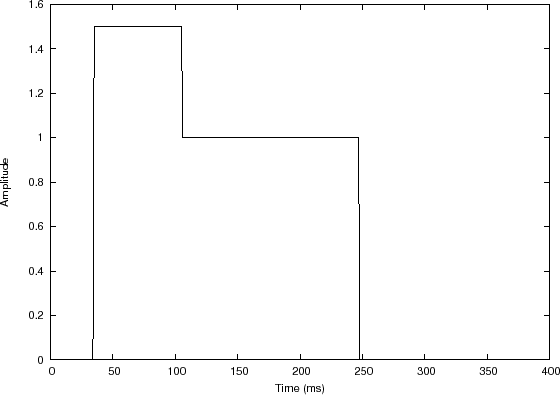
Convolution Example 2: ADSR Envelope
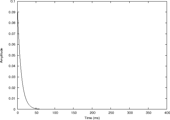
Filter impulse response 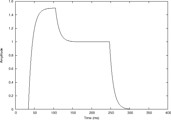
Filter output signal |
In this example, the input signal is a sequence of two rectangular pulses, creating a piecewise constant function, depicted in Fig.7.4(a). The filter impulse response, shown in Fig.7.4(b), is a truncated exponential.7.6
In this example, ![]() is again a causal smoothing-filter impulse
response, and we could call it a ``moving weighted average'', in which
the weighting is exponential into the past. The discontinuous steps
in the input become exponential ``asymptotes'' in the output which are
approached exponentially. The overall appearance of the output signal
resembles what is called an attack, decay, release, and sustain
envelope, or ADSR envelope for short. In a practical ADSR
envelope, the time-constants for attack, decay, and release may be set
independently. In this example, there is only one time constant, that
of
is again a causal smoothing-filter impulse
response, and we could call it a ``moving weighted average'', in which
the weighting is exponential into the past. The discontinuous steps
in the input become exponential ``asymptotes'' in the output which are
approached exponentially. The overall appearance of the output signal
resembles what is called an attack, decay, release, and sustain
envelope, or ADSR envelope for short. In a practical ADSR
envelope, the time-constants for attack, decay, and release may be set
independently. In this example, there is only one time constant, that
of ![]() . The two constant levels in the input signal may be called the
attack level and the sustain level, respectively. Thus,
the envelope approaches the attack level at the attack rate (where the
``rate'' may be defined as the reciprocal of the time constant), it
next approaches the sustain level at the ``decay rate'', and finally,
it approaches zero at the ``release rate''. These envelope parameters
are commonly used in analog synthesizers and their digital
descendants, so-called virtual analog synthesizers. Such an
ADSR envelope is typically used to multiply the output of a waveform
oscillator such as a sawtooth or pulse-train oscillator. For more on
virtual analog synthesis, see, for example,
[78,77].
. The two constant levels in the input signal may be called the
attack level and the sustain level, respectively. Thus,
the envelope approaches the attack level at the attack rate (where the
``rate'' may be defined as the reciprocal of the time constant), it
next approaches the sustain level at the ``decay rate'', and finally,
it approaches zero at the ``release rate''. These envelope parameters
are commonly used in analog synthesizers and their digital
descendants, so-called virtual analog synthesizers. Such an
ADSR envelope is typically used to multiply the output of a waveform
oscillator such as a sawtooth or pulse-train oscillator. For more on
virtual analog synthesis, see, for example,
[78,77].
Convolution Example 3: Matched Filtering
![\includegraphics[width=2.5in]{eps/conv}](http://www.dsprelated.com/josimages_new/mdft/img1185.png)
Figure 7.5 illustrates convolution of
![\begin{eqnarray*}
y&=&[1,1,1,1,0,0,0,0] \\
h&=&[1,0,0,0,0,1,1,1]
\end{eqnarray*}](http://www.dsprelated.com/josimages_new/mdft/img1186.png)
to get
For example,
Graphical Convolution
As mentioned above, cyclic convolution can be written as
Polynomial Multiplication
Note that when you multiply two polynomials together, their
coefficients are convolved. To see this, let ![]() denote the
denote the
![]() th-order polynomial
th-order polynomial
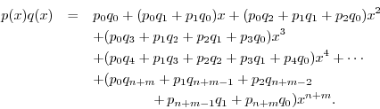
Denoting ![]() by
by
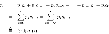
where ![]() and
and ![]() are doubly infinite sequences, defined as
zero for
are doubly infinite sequences, defined as
zero for ![]() and
and ![]() , respectively.
, respectively.
Multiplication of Decimal Numbers
Since decimal numbers are implicitly just polynomials in the powers of 10, e.g.,
Correlation
The correlation operator for two signals ![]() and
and ![]() in
in ![]() is defined as
is defined as
We may interpret the correlation operator as
Stretch Operator
Unlike all previous operators, the
![]() operator maps
a length
operator maps
a length ![]() signal to a length
signal to a length
![]() signal, where
signal, where ![]() and
and ![]() are integers.
We use ``
are integers.
We use ``![]() '' instead of ``
'' instead of ``![]() '' as the time index to underscore this fact.
'' as the time index to underscore this fact.
![\includegraphics[width=4in]{eps/stretch}](http://www.dsprelated.com/josimages_new/mdft/img1216.png)
A stretch by factor ![]() is defined by
is defined by
![$\displaystyle \hbox{\sc Stretch}_{L,m}(x) \isdef
\left\{\begin{array}{ll}
x(...
...x{ an integer} \\ [5pt]
0, & m/L\mbox{ non-integer.} \\
\end{array} \right.
$](http://www.dsprelated.com/josimages_new/mdft/img1217.png)
The stretch operator is used to describe and analyze upsampling,
that is, increasing the sampling rate by an integer factor.
A stretch by ![]() followed by lowpass filtering to the frequency band
followed by lowpass filtering to the frequency band
![]() implements ideal bandlimited interpolation
(introduced in Appendix D).
implements ideal bandlimited interpolation
(introduced in Appendix D).
Zero Padding
Zero padding consists of extending a signal (or spectrum)
with zeros. It maps a length ![]() signal to a length
signal to a length ![]() signal, but
signal, but
![]() need not divide
need not divide ![]() .
.
Definition:
![$\displaystyle \hbox{\sc ZeroPad}_{M,m}(x) \isdef \left\{\begin{array}{ll} x(m),...
...ert m\vert < N/2 \\ [5pt] 0, & \mbox{otherwise} \\ \end{array} \right. \protect$](http://www.dsprelated.com/josimages_new/mdft/img1223.png)
where
Figure 7.7 illustrates zero padding from length ![]() out to length
out to length
![]() . Note that
. Note that ![]() and
and ![]() could be replaced by
could be replaced by ![]() and
and ![]() in the
figure caption.
in the
figure caption.
![\includegraphics[width=\twidth]{eps/zpad}](http://www.dsprelated.com/josimages_new/mdft/img1232.png) |
Note that we have unified the time-domain and frequency-domain
definitions of zero-padding by interpreting the original time axis
![]() as indexing positive-time samples from 0 to
as indexing positive-time samples from 0 to
![]() (for
(for ![]() even), and negative times in the interval
even), and negative times in the interval
![]() .7.8 Furthermore, we require
.7.8 Furthermore, we require
![]() when
when ![]() is even, while odd
is even, while odd ![]() requires no such
restriction. In practice, we often prefer to interpret time-domain
samples as extending from 0 to
requires no such
restriction. In practice, we often prefer to interpret time-domain
samples as extending from 0 to ![]() , i.e., with no negative-time
samples. For this case, we define ``causal zero padding'' as
described below.
, i.e., with no negative-time
samples. For this case, we define ``causal zero padding'' as
described below.
Causal (Periodic) Signals
A signal
![]() may be defined as causal when
may be defined as causal when ![]() for all ``negative-time'' samples (e.g., for
for all ``negative-time'' samples (e.g., for
![]() when
when ![]() is even). Thus, the signal
is even). Thus, the signal
![]() is causal while
is causal while
![]() is not.
For causal signals, zero-padding is equivalent to simply
appending zeros to the original signal. For example,
is not.
For causal signals, zero-padding is equivalent to simply
appending zeros to the original signal. For example,
Causal Zero Padding
In practice, a signal
![]() is often an
is often an ![]() -sample frame of
data taken from some longer signal, and its true starting time can be
anything. In such cases, it is common to treat the start-time of the
frame as zero, with no negative-time samples. In other words,
-sample frame of
data taken from some longer signal, and its true starting time can be
anything. In such cases, it is common to treat the start-time of the
frame as zero, with no negative-time samples. In other words, ![]() represents an
represents an ![]() -sample signal-segment that is translated in time to
start at time 0. In this case (no negative-time samples in the
frame), it is proper to zero-pad by simply appending zeros at the end
of the frame. Thus, we define
e.g.,
-sample signal-segment that is translated in time to
start at time 0. In this case (no negative-time samples in the
frame), it is proper to zero-pad by simply appending zeros at the end
of the frame. Thus, we define
e.g.,
In summary, we have defined two types of zero-padding that arise in practice, which we may term ``causal'' and ``zero-centered'' (or ``zero-phase'', or even ``periodic''). The zero-centered case is the more natural with respect to the mathematics of the DFT, so it is taken as the ``official'' definition of ZEROPAD(). In both cases, however, when properly used, we will have the basic Fourier theorem (§7.4.12 below) stating that zero-padding in the time domain corresponds to ideal bandlimited interpolation in the frequency domain, and vice versa.
Zero Padding Applications
Zero padding in the time domain is used extensively in practice to compute heavily interpolated spectra by taking the DFT of the zero-padded signal. Such spectral interpolation is ideal when the original signal is time limited (nonzero only over some finite duration spanned by the orignal samples).
Note that the time-limited assumption directly contradicts our usual assumption of periodic extension. As mentioned in §6.7, the interpolation of a periodic signal's spectrum from its harmonics is always zero; that is, there is no spectral energy, in principle, between the harmonics of a periodic signal, and a periodic signal cannot be time-limited unless it is the zero signal. On the other hand, the interpolation of a time-limited signal's spectrum is nonzero almost everywhere between the original spectral samples. Thus, zero-padding is often used when analyzing data from a non-periodic signal in blocks, and each block, or frame, is treated as a finite-duration signal which can be zero-padded on either side with any number of zeros. In summary, the use of zero-padding corresponds to the time-limited assumption for the data frame, and more zero-padding yields denser interpolation of the frequency samples around the unit circle.
Sometimes people will say that zero-padding in the time domain yields higher spectral resolution in the frequency domain. However, signal processing practitioners should not say that, because ``resolution'' in signal processing refers to the ability to ``resolve'' closely spaced features in a spectrum analysis (see Book IV [70] for details). The usual way to increase spectral resolution is to take a longer DFT without zero padding--i.e., look at more data. In the field of graphics, the term resolution refers to pixel density, so the common terminology confusion is reasonable. However, remember that in signal processing, zero-padding in one domain corresponds to a higher interpolation-density in the other domain--not a higher resolution.
Ideal Spectral Interpolation
Using Fourier theorems, we will be able to show (§7.4.12) that
zero padding in the time domain gives exact bandlimited interpolation in
the frequency domain.7.9In other words, for truly time-limited signals ![]() ,
taking the DFT of the entire nonzero portion of
,
taking the DFT of the entire nonzero portion of ![]() extended by zeros
yields exact interpolation of the complex spectrum--not an
approximation (ignoring computational round-off error in the DFT
itself). Because the fast Fourier transform (FFT) is so efficient,
zero-padding followed by an FFT is a highly practical method for
interpolating spectra of finite-duration signals, and is used
extensively in practice.
extended by zeros
yields exact interpolation of the complex spectrum--not an
approximation (ignoring computational round-off error in the DFT
itself). Because the fast Fourier transform (FFT) is so efficient,
zero-padding followed by an FFT is a highly practical method for
interpolating spectra of finite-duration signals, and is used
extensively in practice.
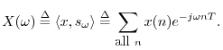
Before we can interpolate a spectrum, we must be clear on what a
``spectrum'' really is. As discussed in Chapter 6, the
spectrum of a signal ![]() at frequency
at frequency ![]() is
defined as a complex number
is
defined as a complex number ![]() computed using the inner
product
computed using the inner
product
Interpolation Operator
The interpolation operator
![]() interpolates a signal
by an integer factor
interpolates a signal
by an integer factor ![]() using bandlimited interpolation. For
frequency-domain signals
using bandlimited interpolation. For
frequency-domain signals
![]() ,
,
![]() , we may
write spectral interpolation as follows:
, we may
write spectral interpolation as follows:
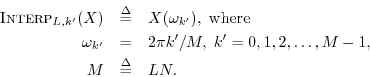
Since
![]() is initially only defined over
the
is initially only defined over
the ![]() roots of unity in the
roots of unity in the ![]() plane, while
plane, while
![]() is defined
over
is defined
over ![]() roots of unity, we define
roots of unity, we define
![]() for
for
![]() by
ideal bandlimited interpolation (specifically time-limited
spectral interpolation in this case).
by
ideal bandlimited interpolation (specifically time-limited
spectral interpolation in this case).
For time-domain signals ![]() , exact interpolation is similarly
bandlimited interpolation, as derived in Appendix D.
, exact interpolation is similarly
bandlimited interpolation, as derived in Appendix D.
Repeat Operator
Like the
![]() and
and
![]() operators, the
operators, the
![]() operator maps a length
operator maps a length ![]() signal to a length
signal to a length
![]() signal:
signal:
Definition: The repeat ![]() times operator is defined for any
times operator is defined for any
![]() by
by
![\includegraphics[width=\twidth]{eps/repeat}](http://www.dsprelated.com/josimages_new/mdft/img1261.png)
A frequency-domain example is shown in Fig.7.9.
Figure 7.9a shows the original spectrum ![]() , Fig.7.9b
shows the same spectrum plotted over the unit circle in the
, Fig.7.9b
shows the same spectrum plotted over the unit circle in the ![]() plane,
and Fig.7.9c shows
plane,
and Fig.7.9c shows
![]() . The
. The ![]() point (dc) is on
the right-rear face of the enclosing box. Note that when viewed as
centered about
point (dc) is on
the right-rear face of the enclosing box. Note that when viewed as
centered about ![]() ,
, ![]() is a somewhat ``triangularly shaped''
spectrum. We see three copies of this shape in
is a somewhat ``triangularly shaped''
spectrum. We see three copies of this shape in
![]() .
.
![\includegraphics[width=4in]{eps/repeat3d}](http://www.dsprelated.com/josimages_new/mdft/img1263.png) |
The repeat operator is used to state the Fourier theorem
Downsampling Operator
Downsampling by ![]() (also called decimation by
(also called decimation by ![]() ) is defined
for
) is defined
for
![]() as taking every
as taking every ![]() th sample, starting with sample zero:
th sample, starting with sample zero:

The
![]() operator maps a length
operator maps a length ![]() signal down to a length
signal down to a length ![]() signal. It is the inverse of the
signal. It is the inverse of the
![]() operator (but not vice
versa), i.e.,
operator (but not vice
versa), i.e.,
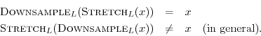
The stretch and downsampling operations do not commute because they are
linear time-varying operators. They can be modeled using
time-varying switches controlled by the sample index ![]() .
.
![\includegraphics[width=4in]{eps/downsamplex}](http://www.dsprelated.com/josimages_new/mdft/img1271.png)
The following example of
![]() is illustrated in Fig.7.10:
is illustrated in Fig.7.10:
Note that the term ``downsampling'' may also refer to the more
elaborate process of sampling-rate conversion to a lower
sampling rate, in which a signal's sampling rate is lowered by resampling
using bandlimited interpolation. To distinguish these cases, we can call
this bandlimited downsampling, because a lowpass-filter is
needed, in general, prior to downsampling so that aliasing is
avoided. This topic is address in Appendix D. Early
sampling-rate converters were in fact implemented using the
![]() operation, followed by an appropriate lowpass filter,
followed by
operation, followed by an appropriate lowpass filter,
followed by
![]() , in order to implement a sampling-rate
conversion by the factor
, in order to implement a sampling-rate
conversion by the factor ![]() .
.
Alias Operator
Aliasing occurs when a signal is undersampled. If the signal
sampling rate ![]() is too low, we get frequency-domain
aliasing.
is too low, we get frequency-domain
aliasing.
The topic of aliasing normally arises in the context of sampling a continuous-time signal. The sampling theorem (Appendix D) says that we will have no aliasing due to sampling as long as the sampling rate is higher than twice the highest frequency present in the signal being sampled.
In this chapter, we are considering only discrete-time signals, in order to keep the math as simple as possible. Aliasing in this context occurs when a discrete-time signal is downsampled to reduce its sampling rate. You can think of continuous-time sampling as the limiting case for which the starting sampling rate is infinity.
An example of aliasing is shown in Fig.7.11. In the figure, the high-frequency sinusoid is indistinguishable from the lower-frequency sinusoid due to aliasing. We say the higher frequency aliases to the lower frequency.
![\includegraphics[scale=0.5]{eps/aliasing}](http://www.dsprelated.com/josimages_new/mdft/img1275.png)
Undersampling in the frequency domain gives rise to time-domain aliasing. If time or frequency is not specified, the term ``aliasing'' normally means frequency-domain aliasing (due to undersampling in the time domain).
The aliasing operator for ![]() -sample signals
-sample signals
![]() is defined by
is defined by
Like the
![]() operator, the
operator, the
![]() operator maps a
length
operator maps a
length ![]() signal down to a length
signal down to a length ![]() signal. A way to think of
it is to partition the original
signal. A way to think of
it is to partition the original ![]() samples into
samples into ![]() blocks of length
blocks of length
![]() , with the first block extending from sample 0 to sample
, with the first block extending from sample 0 to sample ![]() ,
the second block from
,
the second block from ![]() to
to ![]() , etc. Then just add up the blocks.
This process is called aliasing. If the original signal
, etc. Then just add up the blocks.
This process is called aliasing. If the original signal ![]() is
a time signal, it is called time-domain aliasing; if it is a
spectrum, we call it frequency-domain aliasing, or just
aliasing. Note that aliasing is not invertible in general.
Once the blocks are added together, it is usually not possible to
recover the original blocks.
is
a time signal, it is called time-domain aliasing; if it is a
spectrum, we call it frequency-domain aliasing, or just
aliasing. Note that aliasing is not invertible in general.
Once the blocks are added together, it is usually not possible to
recover the original blocks.
Example:
![\begin{eqnarray*}
\hbox{\sc Alias}_2([0,1,2,3,4,5]) &=& [0,1,2] + [3,4,5] = [3,5...
...ox{\sc Alias}_3([0,1,2,3,4,5]) &=& [0,1] + [2,3] + [4,5] = [6,9]
\end{eqnarray*}](http://www.dsprelated.com/josimages_new/mdft/img1280.png)
The alias operator is used to state the Fourier theorem (§7.4.11)
![\includegraphics[width=4.5in]{eps/aliasingfd}](http://www.dsprelated.com/josimages_new/mdft/img1282.png) |
Figure 7.12 shows the result of
![]() applied to
applied to
![]() from Figure 7.9c. Imagine the spectrum of
Fig.7.12a as being plotted on a piece of paper rolled
to form a cylinder, with the edges of the paper meeting at
from Figure 7.9c. Imagine the spectrum of
Fig.7.12a as being plotted on a piece of paper rolled
to form a cylinder, with the edges of the paper meeting at ![]() (upper
right corner of Fig.7.12a). Then the
(upper
right corner of Fig.7.12a). Then the
![]() operation can be
simulated by rerolling the cylinder of paper to cut its circumference in
half. That is, reroll it so that at every point, two sheets of paper
are in contact at all points on the new, narrower cylinder. Now, simply
add the values on the two overlapping sheets together, and you have the
operation can be
simulated by rerolling the cylinder of paper to cut its circumference in
half. That is, reroll it so that at every point, two sheets of paper
are in contact at all points on the new, narrower cylinder. Now, simply
add the values on the two overlapping sheets together, and you have the
![]() of the original spectrum on the unit circle. To alias by
of the original spectrum on the unit circle. To alias by ![]() ,
we would shrink the cylinder further until the paper edges again line up,
giving three layers of paper in the cylinder, and so on.
,
we would shrink the cylinder further until the paper edges again line up,
giving three layers of paper in the cylinder, and so on.
Figure 7.12b shows what is plotted on the first circular wrap of the
cylinder of paper, and Fig.7.12c shows what is on the second wrap.
These are overlaid in Fig.7.12d and added together in
Fig.7.12e. Finally, Figure 7.12f shows both the addition
and the overlay of the two components. We say that the second component
(Fig.7.12c) ``aliases'' to new frequency components, while the
first component (Fig.7.12b) is considered to be at its original
frequencies. If the unit circle of Fig.7.12a covers frequencies
0 to ![]() , all other unit circles (Fig.7.12b-c) cover
frequencies 0 to
, all other unit circles (Fig.7.12b-c) cover
frequencies 0 to ![]() .
.
In general, aliasing by the factor ![]() corresponds to a
sampling-rate reduction by the factor
corresponds to a
sampling-rate reduction by the factor ![]() . To prevent aliasing
when reducing the sampling rate, an anti-aliasing lowpass
filter is generally used. The lowpass filter attenuates all signal
components at frequencies outside the interval
. To prevent aliasing
when reducing the sampling rate, an anti-aliasing lowpass
filter is generally used. The lowpass filter attenuates all signal
components at frequencies outside the interval
![]() so that all frequency components which would alias are first removed.
so that all frequency components which would alias are first removed.
Conceptually, in the frequency domain, the unit circle is reduced by
![]() to a unit circle
half the original size, where the two halves are summed. The inverse
of aliasing is then ``repeating'' which should be understood as
increasing the unit circle circumference using ``periodic
extension'' to generate ``more spectrum'' for the larger unit circle.
In the time domain, on the other hand, downsampling is the inverse of
the stretch operator. We may interchange ``time'' and ``frequency''
and repeat these remarks. All of these relationships are precise only
for integer stretch/downsampling/aliasing/repeat factors; in
continuous time and frequency, the restriction to integer factors is
removed, and we obtain the (simpler) scaling theorem (proved
in §C.2).
to a unit circle
half the original size, where the two halves are summed. The inverse
of aliasing is then ``repeating'' which should be understood as
increasing the unit circle circumference using ``periodic
extension'' to generate ``more spectrum'' for the larger unit circle.
In the time domain, on the other hand, downsampling is the inverse of
the stretch operator. We may interchange ``time'' and ``frequency''
and repeat these remarks. All of these relationships are precise only
for integer stretch/downsampling/aliasing/repeat factors; in
continuous time and frequency, the restriction to integer factors is
removed, and we obtain the (simpler) scaling theorem (proved
in §C.2).
Next Section:
Even and Odd Functions
Previous Section:
The DFT and its Inverse Restated


