


Alternative Wave Variables
We have thus far considered discrete-time simulation of transverse
displacement ![]() in the ideal string. It is equally valid to
choose velocity
in the ideal string. It is equally valid to
choose velocity
![]() , acceleration
, acceleration
![]() , slope
, slope ![]() , or perhaps some other derivative
or integral of displacement with respect to time or position.
Conversion between various time derivatives can be carried out by
means integrators and differentiators, as depicted in
Fig.C.10. Since integration and
differentiation are linear operators, and since the traveling
wave arguments are in units of time, the conversion formulas relating
, or perhaps some other derivative
or integral of displacement with respect to time or position.
Conversion between various time derivatives can be carried out by
means integrators and differentiators, as depicted in
Fig.C.10. Since integration and
differentiation are linear operators, and since the traveling
wave arguments are in units of time, the conversion formulas relating
![]() ,
, ![]() , and
, and ![]() hold also for the traveling wave components
hold also for the traveling wave components
![]() .
.
![\includegraphics[scale=0.9]{eps/fwaveconversions}](http://www.dsprelated.com/josimages_new/pasp/img3445.png) |
Differentiation and integration have a simple form in the
frequency domain. Denoting the Laplace Transform of ![]() by
by
 |
(C.36) |
where ``
| (C.37) |
Similarly,
![\includegraphics[scale=0.9]{eps/ffdwaveconversions}](http://www.dsprelated.com/josimages_new/pasp/img3449.png)
In discrete time, integration and differentiation can be accomplished using digital filters [362]. Commonly used first-order approximations are shown in Fig.C.12.
![\includegraphics[width=\twidth]{eps/fdigitaldiffint}](http://www.dsprelated.com/josimages_new/pasp/img3450.png) |
If discrete-time acceleration ![]() is defined as the sampled version of
continuous-time acceleration, i.e.,
is defined as the sampled version of
continuous-time acceleration, i.e.,
![]() , (for some fixed continuous position
, (for some fixed continuous position ![]() which we
suppress for simplicity of notation), then the
frequency-domain form is given by the
which we
suppress for simplicity of notation), then the
frequency-domain form is given by the ![]() transform
[485]:
transform
[485]:
 |
(C.38) |
In the frequency domain for discrete-time systems, the first-order approximate conversions appear as shown in Fig.C.13.
![\includegraphics[scale=0.6]{eps/ffddigitaldiffint}](http://www.dsprelated.com/josimages_new/pasp/img3454.png) |
The ![]() transform plays the role of the Laplace transform for discrete-time
systems. Setting
transform plays the role of the Laplace transform for discrete-time
systems. Setting ![]() , it can be seen as a sampled Laplace
transform (divided by
, it can be seen as a sampled Laplace
transform (divided by ![]() ), where the sampling is carried out by halting
the limit of the rectangle width at
), where the sampling is carried out by halting
the limit of the rectangle width at ![]() in the definition of a Reimann
integral for the Laplace transform. An important difference between the
two is that the frequency axis in the Laplace transform is the imaginary
axis (the ``
in the definition of a Reimann
integral for the Laplace transform. An important difference between the
two is that the frequency axis in the Laplace transform is the imaginary
axis (the ``![]() axis''), while the frequency axis in the
axis''), while the frequency axis in the ![]() plane is on
the unit circle
plane is on
the unit circle
![]() . As one would expect, the frequency axis for
discrete-time systems has unique information only between frequencies
. As one would expect, the frequency axis for
discrete-time systems has unique information only between frequencies
![]() and
and ![]() while the continuous-time frequency axis extends to plus and
minus infinity.
while the continuous-time frequency axis extends to plus and
minus infinity.
These first-order approximations are accurate (though scaled by ![]() )
at low frequencies relative to half the sampling rate, but they are
not ``best'' approximations in any sense other than being most like
the definitions of integration and differentiation in continuous time.
Much better approximations can be obtained by approaching the problem
from a digital filter design viewpoint, as discussed in §8.6.
)
at low frequencies relative to half the sampling rate, but they are
not ``best'' approximations in any sense other than being most like
the definitions of integration and differentiation in continuous time.
Much better approximations can be obtained by approaching the problem
from a digital filter design viewpoint, as discussed in §8.6.
Spatial Derivatives
In addition to time derivatives, we may apply any number of spatial
derivatives to obtain yet more wave variables to choose from. The first
spatial derivative of string displacement yields slope waves

or, in discrete time,
From this we may conclude that
By the wave equation, curvature waves,
![]() , are
simply a scaling of acceleration waves, in the case of ideal strings.
, are
simply a scaling of acceleration waves, in the case of ideal strings.
In the field of acoustics, the state of a vibrating string at any
instant of time ![]() is often specified by the displacement
is often specified by the displacement
![]() and velocity
and velocity
![]() for all
for all ![]() [317]. Since
velocity is the sum of the traveling velocity waves and
displacement is determined by the difference of the
traveling velocity waves, viz., from Eq.
[317]. Since
velocity is the sum of the traveling velocity waves and
displacement is determined by the difference of the
traveling velocity waves, viz., from Eq.![]() (C.39),
(C.39),
![$\displaystyle y(t,x) \eqsp \int_0^{x} y'(t,\xi)d\xi
\eqsp -\frac{1}{c}\int_0^{x} \left[v_r(t-\xi/c) - v_l(t+\xi/c)\right]d\xi,
$](http://www.dsprelated.com/josimages_new/pasp/img3474.png)
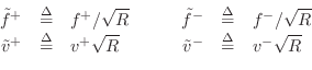
In summary, all traveling-wave variables can be computed from any one, as long as both the left- and right-going component waves are available. Alternatively, any two linearly independent physical variables, such as displacement and velocity, can be used to compute all other wave variables. Wave variable conversions requiring differentiation or integration are relatively expensive since a large-order digital filter is necessary to do it right (§8.6.1). Slope and velocity waves can be computed from each other by simple scaling, and curvature waves are identical to acceleration waves to within a scale factor.
In the absence of factors dictating a specific choice, velocity waves are a good overall choice because (1) it is numerically easier to perform digital integration to get displacement than it is to differentiate displacement to get velocity, (2) slope waves are immediately computable from velocity waves. Slope waves are important because they are a simple scaling of force waves.
Force Waves
![\includegraphics[width=\twidth]{eps/fStringForce}](http://www.dsprelated.com/josimages_new/pasp/img3475.png)
Referring to Fig.C.14, at an arbitrary point ![]() along
the string, the vertical force applied at time
along
the string, the vertical force applied at time ![]() to the portion of
string to the left of position
to the portion of
string to the left of position ![]() by the portion of string to the
right of position
by the portion of string to the
right of position ![]() is given by
is given by
| (C.41) |
assuming
| (C.42) |
These forces must cancel since a nonzero net force on a massless point would produce infinite acceleration. I.e., we must have
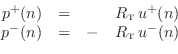
Vertical force waves propagate along the string like any other
transverse wave variable (since they are just slope waves multiplied
by tension ![]() ). We may choose either
). We may choose either ![]() or
or ![]() as the string
force wave variable, one being the negative of the other. It turns
out that to make the description for vibrating strings look the same
as that for air columns, we have to pick
as the string
force wave variable, one being the negative of the other. It turns
out that to make the description for vibrating strings look the same
as that for air columns, we have to pick ![]() , the one that
acts to the right. This makes sense intuitively when one
considers longitudinal pressure waves in an acoustic tube: a
compression wave traveling to the right in the tube pushes the air in
front of it and thus acts to the right. We therefore define the
force wave variable to be
, the one that
acts to the right. This makes sense intuitively when one
considers longitudinal pressure waves in an acoustic tube: a
compression wave traveling to the right in the tube pushes the air in
front of it and thus acts to the right. We therefore define the
force wave variable to be
| (C.43) |
Note that a negative slope pulls up on the segment to the right. At this point, we have not yet considered a traveling-wave decomposition.
Wave Impedance
Using the above identities, we have that the force distribution along the string is given in terms of velocity waves by
![$\displaystyle f(t,x) = \frac{K}{c} \left[{\dot y}_r(t-x/c) - {\dot y}_l(t+x/c) \right], \protect$](http://www.dsprelated.com/josimages_new/pasp/img3483.png)
where
 |
(C.45) |
The wave impedance can be seen as the geometric mean of the two resistances to displacement: tension (spring force) and mass (inertial force).
The digitized traveling force-wave components become
which gives us that the right-going force wave equals the wave impedance times the right-going velocity wave, and the left-going force wave equals minus the wave impedance times the left-going velocity wave.C.4Thus, in a traveling wave, force is always in phase with velocity (considering the minus sign in the left-going case to be associated with the direction of travel rather than a
In the case of the acoustic tube [317,297], we have the analogous relations
 |
(C.47) |
where
| (C.48) |
where
State Conversions
In §C.3.6, an arbitrary string state was converted to traveling displacement-wave components to show that the traveling-wave representation is complete, i.e., that any physical string state can be expressed as a pair of traveling-wave components. In this section, we revisit this topic using force and velocity waves.
By definition of the traveling-wave decomposition, we have
Using Eq.![]() (C.46), we can eliminate
(C.46), we can eliminate
![]() and
and
![]() ,
giving, in matrix form,
,
giving, in matrix form,
![$\displaystyle \left[\begin{array}{c} f \\ [2pt] v \end{array}\right] = \left[\b...
...ay}\right]
\left[\begin{array}{c} f^{{+}} \\ [2pt] f^{{-}} \end{array}\right].
$](http://www.dsprelated.com/josimages_new/pasp/img3492.png)
![$\displaystyle \left[\begin{array}{c} f \\ [2pt] v \end{array}\right] = \left[\b...
...d{array}\right]\left[\begin{array}{c} v^{+} \\ [2pt] v^{-} \end{array}\right].
$](http://www.dsprelated.com/josimages_new/pasp/img3494.png)
Carrying out the inversion to obtain force waves
![]() from
from
![]() yields
yields
![$\displaystyle \left[\begin{array}{c} f^{{+}} \\ [2pt] f^{{-}} \end{array}\right...
...ft[\begin{array}{c} \frac{f+Rv}{2} \\ [2pt] \frac{f-Rv}{2} \end{array}\right].
$](http://www.dsprelated.com/josimages_new/pasp/img3498.png)
![$\displaystyle \left[\begin{array}{c} v^{+} \\ [2pt] v^{-} \end{array}\right] = ...
...[\begin{array}{c} \frac{v+f/R}{2} \\ [2pt] \frac{v-f/R}{2} \end{array}\right].
$](http://www.dsprelated.com/josimages_new/pasp/img3500.png)
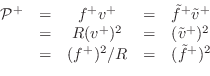
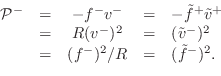
Power Waves
Basic courses in physics teach us that power is work per unit time, and work is a measure of energy which is typically defined as force times distance. Therefore, power is in physical units of force times distance per unit time, or force times velocity. It therefore should come as no surprise that traveling power waves are defined for strings as follows:
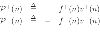 |
From the Ohm's-law relations
![\begin{eqnarray*}
{\cal P}^{+}(n)&=&R[v^{+}(n)]^2 \eqsp [f^{{+}}(n)]^2/R,
\\
{\cal P}^{-}(n)&=&R[v^{-}(n)]^2 \eqsp [f^{{-}}(n)]^2/R.
\end{eqnarray*}](http://www.dsprelated.com/josimages_new/pasp/img3502.png)
Thus, both the left- and right-going components are nonnegative. The sum of the traveling powers at a point gives the total power at that point in the waveguide:
| (C.49) |
If we had left out the minus sign in the definition of left-going power waves, the sum would instead be a net power flow.
Power waves are important because they correspond to the actual ability of the wave to do work on the outside world, such as on a violin bridge at the end of a string. Because energy is conserved in closed systems, power waves sometimes give a simpler, more fundamental view of wave phenomena, such as in conical acoustic tubes. Also, implementing nonlinear operations such as rounding and saturation in such a way that signal power is not increased, gives suppression of limit cycles and overflow oscillations [432], as discussed in the section on signal scattering.
For example, consider a waveguide having a wave impedance which
increases smoothly to the right. A converging cone provides a
practical example in the acoustic tube realm. Then since the energy
in a traveling wave must be in the wave unless it has been transduced
elsewhere, we expect
![]() to propagate unchanged along the
waveguide. However, since the wave impedance is increasing, it must
be true that force is increasing and velocity is decreasing according
to
to propagate unchanged along the
waveguide. However, since the wave impedance is increasing, it must
be true that force is increasing and velocity is decreasing according
to
![]() . Looking only at force or velocity
might give us the mistaken impression that the wave is getting
stronger (looking at force) or weaker (looking at velocity), when
really it was simply sailing along as a fixed amount of energy. This
is an example of a transformer action in which force is
converted into velocity or vice versa. It is well known that a
conical tube acts as if it's open on both ends even though we can
plainly see that it is closed on one end. A tempting explanation is
that the cone acts as a transformer which exchanges pressure and
velocity between the endpoints of the tube, so that a closed end on
one side is equivalent to an open end on the other. However, this
view is oversimplified because, while spherical pressure waves travel
nondispersively in cones, velocity propagation is dispersive
[22,50].
. Looking only at force or velocity
might give us the mistaken impression that the wave is getting
stronger (looking at force) or weaker (looking at velocity), when
really it was simply sailing along as a fixed amount of energy. This
is an example of a transformer action in which force is
converted into velocity or vice versa. It is well known that a
conical tube acts as if it's open on both ends even though we can
plainly see that it is closed on one end. A tempting explanation is
that the cone acts as a transformer which exchanges pressure and
velocity between the endpoints of the tube, so that a closed end on
one side is equivalent to an open end on the other. However, this
view is oversimplified because, while spherical pressure waves travel
nondispersively in cones, velocity propagation is dispersive
[22,50].
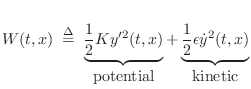
Energy Density Waves
The vibrational energy per unit length along the string, or wave energy density [317] is given by the sum of potential and kinetic energy densities:
 |
(C.50) |
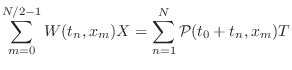
Sampling across time and space, and substituting traveling wave components, one can show in a few lines of algebra that the sampled wave energy density is given by
| (C.51) |
where
![\begin{eqnarray*}
W^{+}(n) &=& \frac{{\cal P}^{+}(n)}{c} \,\mathrel{\mathop=}\,\...
...ht]^2 \,\mathrel{\mathop=}\,\frac{\left[f^{{-}}(n)\right]^2}{K}.
\end{eqnarray*}](http://www.dsprelated.com/josimages_new/pasp/img3508.png)
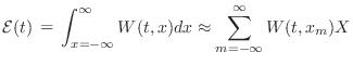
Thus, traveling power waves (energy per unit time)
can be converted to energy density waves (energy per unit length) by
simply dividing by ![]() , the speed of propagation. Quite naturally, the
total wave energy in the string
is given by the integral along the string of the energy density:
, the speed of propagation. Quite naturally, the
total wave energy in the string
is given by the integral along the string of the energy density:
 |
(C.52) |
In practice, of course, the string length is finite, and the limits of integration are from the
Root-Power Waves
It is sometimes helpful to normalize the wave variables so that signal power is uniformly distributed numerically. This can be especially helpful in fixed-point implementations.
From (C.49), it is clear that power normalization is given by
where we have dropped the common time argument `
 |
and
 |
The normalized wave variables
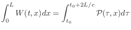
Total Energy in a Rigidly Terminated String
The total energy ![]() in a length
in a length ![]() , rigidly terminated, freely
vibrating string can be computed as
, rigidly terminated, freely
vibrating string can be computed as
 |
(C.54) | ||
 |
(C.55) |
for any
Next Section:
Scattering at Impedance Changes
Previous Section:
The Dispersive 1D Wave Equation


