


Application of the Bilinear Transform
The impedance of a mass in the frequency domain is
![\begin{eqnarray*}
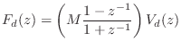
(1+z^{-1})F_d(z) &=& M (1-z^{-1}) V_d(z) \\
\;\longleftrighta...
...
\,\,\Rightarrow\,\,f_d(n) &=& M[v_d(n) - v_d(n-1)] - f_d(n-1).
\end{eqnarray*}](http://www.dsprelated.com/josimages_new/pasp/img1686.png)
This difference equation is diagrammed in Fig. 7.16. We recognize this recursive digital filter as the direct form I structure. The direct-form II structure is obtained by commuting the feedforward and feedback portions and noting that the two delay elements contain the same value and can therefore be shared [449]. The two other major filter-section forms are obtained by transposing the two direct forms by exchanging the input and output, and reversing all arrows. (This is a special case of Mason's Gain Formula which works for the single-input, single-output case.) When a filter structure is transposed, its summers become branching nodes and vice versa. Further discussion of the four basic filter section forms can be found in [333].
![\includegraphics[width=4in]{eps/lmassFilterDF1}](http://www.dsprelated.com/josimages_new/pasp/img1687.png) |
Practical Considerations
While the digital mass simulator has the desirable properties of the bilinear transform,
it is also not perfect from a practical point of view:
(1) There is a pole at half the sampling rate (![]() ).
(2) There is a delay-free path from input to output.
).
(2) There is a delay-free path from input to output.
The first problem can easily be circumvented by introducing a loss factor ![]() ,
moving the pole from
,
moving the pole from ![]() to
to ![]() , where
, where ![]() and
and ![]() . This
is sometimes called the ``leaky integrator''.
. This
is sometimes called the ``leaky integrator''.
The second problem arises when making loops of elements (e.g., a mass-spring chain which forms a loop). Since the individual elements have no delay from input to output, a loop of elements is not computable using standard signal processing methods. The solution proposed by Alfred Fettweis is known as ``wave digital filters,'' a topic taken up in §F.1.
Next Section:
Limitations of Lumped Element Digitization
Previous Section:
Bilinear Transformation


