


Boundary Conditions
The relations of the previous section do not hold exactly when the string length is finite. A finite-length string forces consideration of boundary conditions. In this section, we will introduce boundary conditions as perturbations of the state transition matrix. In addition, we will use the DW-FDTD equivalence to obtain physically well behaved boundary conditions for the FDTD method.
Consider an ideal vibrating string with ![]() spatial samples. This is a sufficiently large number to make clear
most of the repeating patterns in the general case. Introducing
boundary conditions is most straightforward in the DW paradigm. We
therefore begin with the order 8 DW model, for which the state vector
(for the 0th subgrid) will be
spatial samples. This is a sufficiently large number to make clear
most of the repeating patterns in the general case. Introducing
boundary conditions is most straightforward in the DW paradigm. We
therefore begin with the order 8 DW model, for which the state vector
(for the 0th subgrid) will be
![\begin{displaymath}
\underline{x}_W(n) =
\left[\!
\begin{array}{l}
y^{+}_{n,0}\...
...}_{n,4}\\
y^{+}_{n,6}\\
y^{-}_{n,6}\\
\end{array}\!\right].
\end{displaymath}](http://www.dsprelated.com/josimages_new/pasp/img4678.png)
![\begin{displaymath}
\mathbf{C}_W=
\left[\!
\begin{array}{ccccccccccc}
1 & 1 & ...
...0 & 0 \\
0 & 0 & 0 & 0 & 0 & 0 & 1 & 1
\end{array}\!\right]
\end{displaymath}](http://www.dsprelated.com/josimages_new/pasp/img4679.png)
![\begin{displaymath}
{\mathbf{B}_W}
=
\left[\!
\begin{array}{cc}
0 & 0 \\
0 & ...
...
0 & 0 \\
0 & 0 \\
0 & 0 \\
0 & 0
\end{array}\!\right]
\end{displaymath}](http://www.dsprelated.com/josimages_new/pasp/img4681.png)
Resistive Terminations
Let's begin with simple ``resistive'' terminations at the string
endpoints, resulting in the reflection coefficient ![]() at each end of
the string, where
at each end of
the string, where
![]() corresponds to nonnegative (passive)
termination resistances [447]. Inspection of
Fig.E.2 makes it clear that terminating the left endpoint may be
accomplished by setting
corresponds to nonnegative (passive)
termination resistances [447]. Inspection of
Fig.E.2 makes it clear that terminating the left endpoint may be
accomplished by setting
![$\displaystyle \tilde{\mathbf{A}}_W= \left[\! \begin{array}{ccccccccccc} 0 & g_l...
... 0 & 0 & 1 & 0 & 0 & 0 \\ 0 & 0 & 0 & 0 & 0 & 0 & g_r & 0 \end{array} \!\right]$](http://www.dsprelated.com/josimages_new/pasp/img4684.png) |
(E.38) |
The simplest choice of state transformation matrix
![\begin{displaymath}
\mathbf{T}\isdef
\left[\!
\begin{array}{ccccccccccc}
1 & 1...
... 1 & 1 \\
0 & 0 & 0 & 0 & 0 & 0 & 0 & 1
\end{array}\!\right]
\end{displaymath}](http://www.dsprelated.com/josimages_new/pasp/img4685.png)
![\begin{eqnarray*}
\tilde{\mathbf{A}}_K&\isdef & \mathbf{T}\tilde{\mathbf{A}}_W\m...
...r \\
0 & 0 & 0 & 0 & 0 & 0 & g_r & -g_r
\end{array}\!\right],
\end{eqnarray*}](http://www.dsprelated.com/josimages_new/pasp/img4687.png)
where
![]() and
and
![]() . We see that the left
FDTD termination is non-local for
. We see that the left
FDTD termination is non-local for ![]() , while the right
termination is local (to two adjacent spatial samples) for all
, while the right
termination is local (to two adjacent spatial samples) for all ![]() .
This can be viewed as a consequence of having ordered the FDTD state
variables as
.
This can be viewed as a consequence of having ordered the FDTD state
variables as
![]() instead of
instead of
![]() . Choosing the other ordering
interchanges the endpoint behavior. Call these orderings Type I and
Type II, respectively. Then
. Choosing the other ordering
interchanges the endpoint behavior. Call these orderings Type I and
Type II, respectively. Then
![]() ; that is, the similarity
transformation matrix
; that is, the similarity
transformation matrix
![]() is transposed when converting from Type I
to Type II or vice versa. By anechoically coupling a Type I FDTD
simulation on the right with a Type II simulation on the left,
general resistive terminations may be obtained on both ends which are
localized to two spatial samples.
is transposed when converting from Type I
to Type II or vice versa. By anechoically coupling a Type I FDTD
simulation on the right with a Type II simulation on the left,
general resistive terminations may be obtained on both ends which are
localized to two spatial samples.
In nearly all musical sound synthesis applications, at least one of
the string endpoints is modeled as rigidly clamped at the ``nut''.
Therefore, since the FDTD, as defined here, most naturally provides
a clamped endpoint on the left, with more general localized terminations
possible on the right, we will proceed with this case for simplicity in what
follows. Thus, we set ![]() and obtain
and obtain
![\begin{eqnarray*}
\mbox{$\stackrel{{\scriptscriptstyle \vdash}}{\mathbf{A}}$}_K&...
..._r \\
0 & 0 & 0 & 0 & 0 & 0 & g_r & -g_r
\end{array}\!\right]
\end{eqnarray*}](http://www.dsprelated.com/josimages_new/pasp/img4695.png)
Boundary Conditions as Perturbations
To study the effect of boundary conditions on the state transition
matrices
![]() and
and
![]() , it is convenient to write the terminated
transition matrix as the sum of of the ``left-clamped'' case
, it is convenient to write the terminated
transition matrix as the sum of of the ``left-clamped'' case
![]()
![]() (for which
(for which ![]() ) plus a series of one or more rank-one
perturbations. For example, introducing a right termination with
reflectance
) plus a series of one or more rank-one
perturbations. For example, introducing a right termination with
reflectance ![]() can be written
can be written
where
In general, when ![]() is odd, adding
is odd, adding
![]() to
to
![]()
![]() corresponds to a connection from left-going waves to
right-going waves, or vice versa (see Fig.E.2). When
corresponds to a connection from left-going waves to
right-going waves, or vice versa (see Fig.E.2). When ![]() is
odd and
is
odd and ![]() is even, the connection flows from the right-going to the
left-going signal path, thus providing a termination (or partial
termination) on the right. Left terminations flow from the bottom to
the top rail in Fig.E.2, and in such connections
is even, the connection flows from the right-going to the
left-going signal path, thus providing a termination (or partial
termination) on the right. Left terminations flow from the bottom to
the top rail in Fig.E.2, and in such connections ![]() is even
and
is even
and ![]() is odd. The spatial sample numbers involved in the connection
are
is odd. The spatial sample numbers involved in the connection
are
![]() and
and
![]() , where
, where
![]() denotes the greatest integer less than or equal to
denotes the greatest integer less than or equal to
![]() .
.
The rank-one perturbation of the DW transition matrix Eq.![]() (E.39)
corresponds to the following rank-one perturbation of the FDTD
transition matrix
(E.39)
corresponds to the following rank-one perturbation of the FDTD
transition matrix
![]()
![]() :
:
![\begin{displaymath}\mathbf{T}{\bm \delta}_{8,7}\mathbf{T}^{-1}
=
\left[\!
\begin...
...
0 & 0 & 0 & 0 & 0 & 0 & 1 & -1
\end{array}\!\right].
\protect\end{displaymath}](http://www.dsprelated.com/josimages_new/pasp/img4713.png)
In general, we have
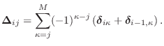
Thus, the general rule is that
Reactive Terminations
In typical string models for virtual musical instruments, the ``nut
end'' of the string is rigidly clamped while the ``bridge end'' is
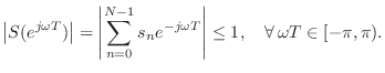
terminated in a passive reflectance ![]() . The condition
for passivity of the reflectance is simply that its gain be bounded
by 1 at all frequencies [447]:
. The condition
for passivity of the reflectance is simply that its gain be bounded
by 1 at all frequencies [447]:
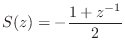
A very simple case, used, for example, in the Karplus-Strong plucked-string algorithm, is the two-point-average filter:
![\begin{eqnarray*}
\mbox{$\stackrel{{\scriptscriptstyle \vdash\!\!\dashv}}{\mathb...
... \\
0 & 0 & 0 & 0 & -1/2 & 1/2 & -1 & -1
\end{array}\!\right].
\end{eqnarray*}](http://www.dsprelated.com/josimages_new/pasp/img4722.png)
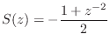
This gives the desired filter in a half-rate, staggered grid case. In the full-rate case, the termination filter is really
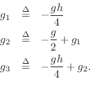
Another often-used string termination filter in digital waveguide models is specified by [447]
![\begin{eqnarray*}
s(n) &=& -g\left[\frac{h}{4}, \frac{1}{2}, \frac{h}{4}\right]\...
...{j\omega T})&=&
-e^{-j\omega T}g\frac{1 + h \cos(\omega T)}{2},
\end{eqnarray*}](http://www.dsprelated.com/josimages_new/pasp/img4724.png)
where ![]() is an overall gain factor that affects the decay
rate of all frequencies equally, while
is an overall gain factor that affects the decay
rate of all frequencies equally, while ![]() controls the
relative decay rate of low-frequencies and high frequencies. An
advantage of this termination filter is that the delay is
always one sample, for all frequencies and for all parameter settings;
as a result, the tuning of the string is invariant with respect to
termination filtering. In this case, the perturbation is
controls the
relative decay rate of low-frequencies and high frequencies. An
advantage of this termination filter is that the delay is
always one sample, for all frequencies and for all parameter settings;
as a result, the tuning of the string is invariant with respect to
termination filtering. In this case, the perturbation is
![\begin{eqnarray*}
\mbox{$\stackrel{{\scriptscriptstyle \vdash\!\!\dashv}}{\mathb...
...d g_2 & \quad -g_2 & \quad g_3 & \quad -g_3
\end{array}\!\right]
\end{eqnarray*}](http://www.dsprelated.com/josimages_new/pasp/img4728.png)
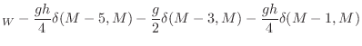
where
The filtered termination examples of this section generalize
immediately to arbitrary finite-impulse response (FIR) termination
filters ![]() . Denote the impulse response of the termination filter
by
. Denote the impulse response of the termination filter
by
Interior Scattering Junctions
A so-called Kelly-Lochbaum scattering junction [297,447] can be introduced into the string at the fourth sample by the following perturbation
A single time-varying scattering junction provides a reasonable model for plucking, striking, or bowing a string at a point. Several adjacent scattering junctions can model a distributed interaction, such as a piano hammer, finger, or finite-width bow spanning several string samples.
Note that scattering junctions separated by one spatial sample (as
typical in ``digital waveguide filters'' [447]) will
couple the formerly independent subgrids. If scattering junctions are
confined to one subgrid, they are separated by two samples of delay
instead of one, resulting in round-trip transfer functions of the form
![]() (as occurs in the digital waveguide mesh). In the context of
a half-rate staggered-grid scheme, they can provide general IIR
filtering in the form of a ladder digital filter [297,447].
(as occurs in the digital waveguide mesh). In the context of
a half-rate staggered-grid scheme, they can provide general IIR
filtering in the form of a ladder digital filter [297,447].
Next Section:
Lossy Vibration
Previous Section:
DW State Space Model


