


Digital Waveguide Modeling Elements
As mentioned above, digital waveguide models are built out of digital delay-lines and filters (and nonlinear elements), and they can be understood as propagating and filtering sampled traveling-wave solutions to the wave equation (PDE), such as for air, strings, rods, and the like [433,437]. It is noteworthy that strings, woodwinds, and brasses comprise three of the four principal sections of a classical orchestra (all but percussion). The digital waveguide modeling approach has also been extended to propagation in 2D, 3D, and beyond [518,396,522,400]. They are not finite-difference models, but paradoxically they are equivalent under certain conditions (Appendix E). A summary of historical aspects appears in §A.9.
As mentioned at Eq.![]() (1.1), the ideal wave equation comes directly
from Newton's laws of motion (
(1.1), the ideal wave equation comes directly
from Newton's laws of motion (![]() ). For example, in the case of
vibrating strings, the wave equation is derived from first principles
(in Chapter 6, and more completely in Appendix C) to
be
). For example, in the case of
vibrating strings, the wave equation is derived from first principles
(in Chapter 6, and more completely in Appendix C) to
be
![\begin{eqnarray*}
Ky''&=& \epsilon {\ddot y}\\ [5pt]
\mbox{(Restoring Force Density} &=& \mbox{Mass Density times
Acceleration)}, \end{eqnarray*}](http://www.dsprelated.com/josimages_new/pasp/img369.png)
where
Defining
![]() , we obtain the usual form of the PDE known as
the ideal 1D wave equation.
, we obtain the usual form of the PDE known as
the ideal 1D wave equation.
where
![\begin{eqnarray*}
{\ddot y}& \isdef & \frac{\partial^2}{\partial t^2} y(t,x)\\ [5pt]
y''& \isdef & \frac{\partial^2}{\partial x^2} y(t,x).
\end{eqnarray*}](http://www.dsprelated.com/josimages_new/pasp/img375.png)
As has been known since d'Alembert [100], the 1D wave
equation is obeyed by arbitrary traveling waves at speed ![]() :
:
In digital waveguide modeling, the traveling-waves are sampled:
![\begin{eqnarray*}
y(nT,mX)
&=& y_r(nT-mX/c) + y_l(nT+mX/c)\qquad \mbox{(set $X=...
...y_r(nT-mT) + y_l(nT+mT)\\ [5pt]
&\isdef &y^{+}(n-m) + y^{-}(n+m)
\end{eqnarray*}](http://www.dsprelated.com/josimages_new/pasp/img379.png)
where ![]() denotes the time sampling interval in seconds,
denotes the time sampling interval in seconds, ![]() denotes the spatial sampling interval in meters, and
denotes the spatial sampling interval in meters, and ![]() and
and ![]() are defined for notational convenience.
are defined for notational convenience.
An ideal string (or air column) can thus be simulated using a
bidirectional delay line, as shown in
Fig.1.13 for the case of an ![]() -sample
section of ideal string or air column. The ``
-sample
section of ideal string or air column. The ``![]() '' label denotes its
wave impedance (§6.1.5) which is needed when connecting
digital waveguides to each other and to other kinds of computational
physical models (such as finite difference schemes). While
propagation speed on an ideal string is
'' label denotes its
wave impedance (§6.1.5) which is needed when connecting
digital waveguides to each other and to other kinds of computational
physical models (such as finite difference schemes). While
propagation speed on an ideal string is
![]() , we will
derive (§C.7.3) that the wave impedance is
, we will
derive (§C.7.3) that the wave impedance is
![]() .
.
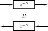 |
Figure 1.14 (from Chapter 6,
§6.3), illustrates a simple digital waveguide model for
rigidly terminated vibrating strings (more specifically, one
polarization-plane of transverse vibration). The traveling-wave
components are taken to be displacement samples, but the
diagram for velocity-wave and acceleration-wave simulation are
identical (inverting reflection at each rigid termination). The
output signal ![]() is formed by summing traveling-wave
components at the desired ``virtual pickup'' location (position
is formed by summing traveling-wave
components at the desired ``virtual pickup'' location (position
![]() in this example). To drive the string at a particular point,
one simply takes the transpose [449] of the output sum,
i.e., the input excitation is summed equally into the left- and
right-going delay-lines at the same
in this example). To drive the string at a particular point,
one simply takes the transpose [449] of the output sum,
i.e., the input excitation is summed equally into the left- and
right-going delay-lines at the same ![]() position (details will be
discussed near Fig.6.14).
position (details will be
discussed near Fig.6.14).
![\includegraphics[width=\twidth]{eps/fterminatedstringCopy}](http://www.dsprelated.com/josimages_new/pasp/img386.png) |
In Chapter 9 (example applications), we will discuss digital waveguide models for single-reed instruments such as the clarinet (Fig.1.15), and bowed-string instruments (Fig.1.16) such as the violin.
![\includegraphics[width=\twidth]{eps/fSingleReedWGMCopy}](http://www.dsprelated.com/josimages_new/pasp/img387.png) |
![\includegraphics[width=\twidth]{eps/fBowedStringsWGMCopy}](http://www.dsprelated.com/josimages_new/pasp/img388.png)
Next Section:
General Modeling Procedure
Previous Section:
Wave Digital Filters


