Eigenstructure

Free Books Physical Audio Signal Processing

Starting with the defining equation for an eigenvector $\underline{e}$ and its corresponding eigenvalue $\lambda$ ,

$\displaystyle \mathbf{A}\underline{e}_i = {\lambda_i}\underline{e}_i,\quad i=1,2$

we get, using Eq. $\,$ (C.137),

$\displaystyle \left[\begin{array}{cc} gc & c-1 \\ [2pt] gc+g & c \end{array}\ri... ...n{array}{c} {\lambda_i} \\ [2pt] {\lambda_i}\eta_i \end{array}\right]. \protect$

(C.140)

We normalized the first element of $\underline{e}_i$ to 1 since $g\underline{e}_i$ is an eigenvector whenever $\underline{e}_i$ is. (If there is a missing solution because its first element happens to be zero, we can repeat the analysis normalizing the second element to 1 instead.)

Equation (C.141) gives us two equations in two unknowns:

$\displaystyle gc+\eta_i(c-1)$	$\displaystyle =$	$\displaystyle {\lambda_i} \protect$	(C.141)
$\displaystyle g(1+c) +c\eta_i$	$\displaystyle =$	$\displaystyle {\lambda_i}\eta_i$	(C.142)

Substituting the first into the second to eliminate ${\lambda_i}$ , we get

$\begin{eqnarray*} g+gc+c\eta_i &=& [gc+\eta_i(c-1)]\eta_i = gc\eta_i + \eta_i^2 ... ...{g\left(\frac{1+c}{1-c}\right) - \frac{c^2(1-g)^2}{4(1-c)^2}}. \end{eqnarray*}$

As approaches (no damping), we obtain

$\displaystyle \eta_i = \pm j\sqrt{\frac{1+c}{1-c}} \qquad \hbox{(when $g=1$)}.$

Thus, we have found both eigenvectors:

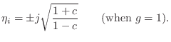
$\begin{eqnarray*} \underline{e}_1&=&\left[\begin{array}{c} 1 \\ [2pt] \eta \end{... ...t{g\left(\frac{1+c}{1-c}\right) - \frac{c^2(1-g)^2}{4(1-c)^2}} \end{eqnarray*}$

They are linearly independent provided $\eta\neq0$ . In the undamped case (), this holds whenever $c\neq -1$ . The eigenvectors are finite when $c\neq 1$ . Thus, the nominal range for is the interval $c\in(-1,1)$ .

We can now use Eq. $\,$ (C.142) to find the eigenvalues:

$\begin{eqnarray*} {\lambda_i}&=& gc+ \eta_i(c-1)\\ &=& gc+ \frac{(1-g)c}{2}\pm ... ... \pm j\sqrt{g(1-c^2) - \left[\frac{c(1-g)}{2}\right]^2} \protect \end{eqnarray*}$

Damping and Tuning Parameters

The tuning and damping of the resonator impulse response are governed by the relation

$\displaystyle {\lambda_i}= e^{\frac{T}{\tau}} e^{\pm j\omega T}$

where

denotes the sampling interval, $\tau$ is the time constant of decay, and $\omega$ is the frequency of oscillation in radians per second. The eigenvalues are presumed to be complex, which requires, from Eq. $\,$ (C.144),

$\displaystyle g(1-c^2) \geq\frac{c^2(1-g)^2}{4} \,\,\Rightarrow\,\,c^2 \leq \frac{4g}{(1+g)^2}$

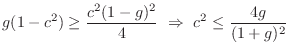
To obtain a specific decay time-constant $\tau$ , we must have

$\begin{eqnarray*} e^{-2T/\tau} &=& \left\vert{\lambda_i}\right\vert^2 = c^2\left... ...left[g(1-c^2) - c^2\left(\frac{1-g}{2}\right)^2\right]\\ &=& g \end{eqnarray*}$

Therefore, given a desired decay time-constant $\tau$ (and the sampling interval ), we may compute the damping parameter for the digital waveguide resonator as

$\displaystyle \zbox {g = e^{-2T/\tau}.}$

Note that this conclusion follows directly from the determinant analysis of Eq. $\,$ (C.140), provided it is known that the poles form a complex-conjugate pair.

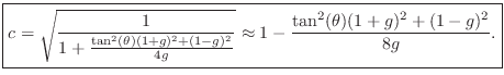
To obtain a desired frequency of oscillation, we must solve

$\begin{eqnarray*} \theta = \omega T &=& \tan^{-1}\left[\frac{\sqrt{g(1-c^2) - [... ...,\tan^2{\theta} &=& \frac{g(1-c^2) - [c(1-g)/2]^2}{[c(1+g)/2]^2} \end{eqnarray*}$

for , which yields

$\displaystyle \zbox { c= \sqrt{\frac{1}{1 + \frac{\tan^2(\theta)(1+g)^2+(1-g)^2}{4g}}} \approx 1 - \frac{\tan^2(\theta)(1+g)^2 + (1-g)^2}{8g}. }$

Note that this reduces to $c=\cos(\theta)$ when

(undamped case).

Eigenvalues in the Undamped Case

When , the eigenvalues reduce to

$\displaystyle {\lambda_i}= c\pm j\sqrt{1-c^2}$

Assuming $\left\vert c\right\vert<1$ , the eigenvalues can be expressed as

$\displaystyle {\lambda_i}= c\pm j\sqrt{1-c^2} = \cos(\theta) \pm j\sin(\theta) = e^{\pm j\theta} \protect$

(C.143)

where $\theta=\omega T$ denotes the angular advance per sample of the oscillator. Since $c\in(-1,1)$ corresponds to the range $\theta\in(-\pi,\pi)$ , we see that

in this range can produce oscillation at any digital frequency.

For $\left\vert c\right\vert>1$ , the eigenvalues are real, corresponding to exponential growth and/or decay. (The values $c=\pm 1$ were excluded above in deriving Eq. $\,$ (C.144).)