Beginning with a restatement of Eq. (4.9),
we can express each FIR coefficient

as a vector
expression:
Making a row-vector out of the FIR coefficients gives
or
We may now choose a set of parameter values
![$ {\underline{\Delta}}^T=[\Delta_0,\Delta_1,\ldots,\Delta_L]$](http://www.dsprelated.com/josimages_new/pasp/img1093.png)
over which an optimum approximation is desired, yielding
the
matrix equation
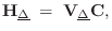 |
(5.11) |
where
![$\displaystyle \mathbf{H}_{\underline{\Delta}}\isdefs \left[\begin{array}{c} \un...
...elta_0}^T \\ [2pt] \vdots \\ [2pt] \underline{h}_{\Delta_L}^T\end{array}\right]$](http://www.dsprelated.com/josimages_new/pasp/img1095.png)
and
![$\displaystyle \qquad
\mathbf{V}_{\underline{\Delta}}\isdefs \left[\begin{array}...
...ta_0}^T \\ [2pt] \vdots \\ [2pt] \underline{V}_{\Delta_L}^T\end{array}\right].
$](http://www.dsprelated.com/josimages_new/pasp/img1096.png)
Equation (
4.11) may be solved for the polynomial-coefficient
matrix

by usual
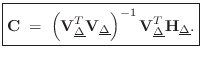
least-squares methods. For example, in the unweighted
case, with

, we have
Note that this formulation is valid for finding the Farrow
coefficients of any

th-order variable
FIR filter parametrized by a
single variable

.
Lagrange interpolation is a special case
corresponding to a particular choice of

.
Next Section: Differentiator Filter BankPrevious Section: Farrow Structure

![$\displaystyle h_\Delta(n) \eqsp
\underbrace{%
\left[\begin{array}{ccccc} 1 & \...
...y}{c} C_n(0) \\ [2pt] C_n(1) \\ [2pt] \vdots \\ [2pt] C_n(M)\end{array}\right]
$](http://www.dsprelated.com/josimages_new/pasp/img1090.png)
![$\displaystyle \underbrace{\left[\begin{array}{cccc}h_\Delta(0)\!&\!h_\Delta(1)\...
...\vdots \\
C_0(M) & C_1(M) & \cdots & C_N(M)
\end{array}\right]}_{\mathbf{C}}
$](http://www.dsprelated.com/josimages_new/pasp/img1091.png)