DSPRelated.com
Free Books

General Nonlinear ODE

In state-space form (§1.3.7) [449],8.7a general class of $ N$th-order Ordinary Differential Equations (ODE), can be written as

$\displaystyle \dot{\underline{x}}(t) \eqsp f(t,\underline{x},\underline{u}) \protect$ (8.8)

where $ t$ denotes time in seconds, $ \underline{x}(t)$ denotes a vector of $ N$ state variables at time $ t$,

$\displaystyle \dot{\underline{x}}(t) \isdefs \frac{d}{dt}\underline{x}(t)
$

denotes the time derivative of $ \underline{x}(t)$, and $ \underline{u}(t)$ is a vector (any length) of the system input signals, if any. Thus, Eq.$ \,$(7.8) says simply that the time-derivative of the state vector is some function $ f$ depending on time $ t$, the current state $ \underline{x}(t)$, and the current input signals $ \underline{u}(t)$. The basic problem is to solve for the state trajectory $ \underline{x}(t)$ given its initial condition $ \underline{x}(0)$, the system definition function $ f$, and the input signals $ \underline{u}(t)$ for all $ t\ge 0$.

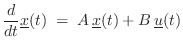
In the linear, time-invariant (LTI) case, Eq.$ \,$(7.8) can be expressed in the usual state-space form for LTI continuous-time systems:

$\displaystyle \frac{d}{dt}\underline{x}(t) \eqsp A\,\underline{x}(t) + B\,\underline{u}(t) \protect$ (8.9)

In this case, standard methods for converting a filter from continuous to discrete time may be used, such as the FDA7.3.1) and bilinear transform7.3.2).8.8


Next Section:
Forward Euler Method
Previous Section:
Limitations of Lumped Element Digitization