


Linear Interpolation as Resampling
Convolution Interpretation
Linearly interpolated fractional delay is equivalent to filtering and resampling a weighted impulse train (the input signal samples) with a continuous-time filter having the simple triangular impulse response
![$\displaystyle h_l(t) = \left\{\begin{array}{ll} 1-\left\vert t/T\right\vert, & ...
...ght\vert\leq T, \\ [5pt] 0, & \hbox{otherwise}. \\ \end{array} \right. \protect$](http://www.dsprelated.com/josimages_new/pasp/img959.png)
Convolution of the weighted impulse train with
This continuous result can then be resampled at the desired fractional delay.
In discrete time processing, the operation Eq.![]() (4.5) can be
approximated arbitrarily closely by digital upsampling by a
large integer factor
(4.5) can be
approximated arbitrarily closely by digital upsampling by a
large integer factor ![]() , delaying by
, delaying by ![]() samples (an integer), then
finally downsampling by
samples (an integer), then
finally downsampling by ![]() , as depicted in Fig.4.7
[96]. The integers
, as depicted in Fig.4.7
[96]. The integers ![]() and
and ![]() are chosen so that
are chosen so that
![]() , where
, where ![]() the desired fractional delay.
the desired fractional delay.
![\includegraphics[width=0.8\twidth]{eps/polyphaseli}](http://www.dsprelated.com/josimages_new/pasp/img963.png)
The convolution interpretation of linear interpolation, Lagrange interpolation, and others, is discussed in [407].
Frequency Response of Linear Interpolation
Since linear interpolation can be expressed as a convolution of the
samples with a triangular pulse, we can derive the frequency
response of linear interpolation. Figure 4.7 indicates that
the triangular pulse ![]() serves as an anti-aliasing lowpass
filter for the subsequent downsampling by
serves as an anti-aliasing lowpass
filter for the subsequent downsampling by ![]() . Therefore, it should
ideally ``cut off'' all frequencies higher than
. Therefore, it should
ideally ``cut off'' all frequencies higher than ![]() .
.
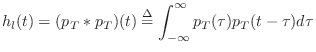
Triangular Pulse as Convolution of Two Rectangular Pulses
The 2-sample wide triangular pulse ![]() (Eq.
(Eq.![]() (4.4)) can be
expressed as a convolution of the one-sample rectangular pulse with
itself.
(4.4)) can be
expressed as a convolution of the one-sample rectangular pulse with
itself.
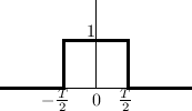
The one-sample rectangular pulse is shown in Fig.4.8 and may be defined analytically as
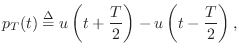
![$\displaystyle u(t) \isdef \left\{\begin{array}{ll}
1, & t\geq 0 \\ [5pt]
0, & t<0 \\
\end{array}\right..
$](http://www.dsprelated.com/josimages_new/pasp/img968.png)
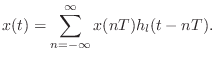
Linear Interpolation Frequency Response
Since linear interpolation is a convolution of the samples with a
triangular pulse
![]() (from Eq.
(from Eq.![]() (4.5)),
the frequency response of the interpolation is given by the Fourier
transform
(4.5)),
the frequency response of the interpolation is given by the Fourier
transform ![]() , which yields a
sinc
, which yields a
sinc![]() function. This frequency
response applies to linear interpolation from discrete time to
continuous time. If the output of the interpolator is also sampled,
this can be modeled by sampling the continuous-time interpolation
result in Eq.
function. This frequency
response applies to linear interpolation from discrete time to
continuous time. If the output of the interpolator is also sampled,
this can be modeled by sampling the continuous-time interpolation
result in Eq.![]() (4.5), thereby aliasing the
sinc
(4.5), thereby aliasing the
sinc![]() frequency
response, as shown in Fig.4.9.
frequency
response, as shown in Fig.4.9.
![\includegraphics[width=3in]{eps/sincsquared}](http://www.dsprelated.com/josimages_new/pasp/img979.png)
In slightly more detail, from
![]() , and
, and
![]() sinc
sinc![]() , we have
, we have
The Fourier transform of ![]() is the same function aliased on
a block of size
is the same function aliased on
a block of size ![]() Hz. Both
Hz. Both ![]() and its alias are plotted
in Fig.4.9. The example in this figure pertains to an
output sampling rate which is
and its alias are plotted
in Fig.4.9. The example in this figure pertains to an
output sampling rate which is ![]() times that of the input signal.
In other words, the input signal is upsampled by a factor of
times that of the input signal.
In other words, the input signal is upsampled by a factor of ![]() using linear interpolation. The ``main lobe'' of the interpolation
frequency response
using linear interpolation. The ``main lobe'' of the interpolation
frequency response ![]() contains the original signal bandwidth;
note how it is attenuated near half the original sampling rate (
contains the original signal bandwidth;
note how it is attenuated near half the original sampling rate (![]() in Fig.4.9). The ``sidelobes'' of the frequency response
contain attenuated copies of the original signal bandwidth (see
the DFT stretch theorem), and thus constitute spectral imaging
distortion in the final output (sometimes also referred to as a kind
of ``aliasing,'' but, for clarity, that term will not be used for
imaging distortion in this book). We see that the frequency response
of linear interpolation is less than ideal in two ways:
in Fig.4.9). The ``sidelobes'' of the frequency response
contain attenuated copies of the original signal bandwidth (see
the DFT stretch theorem), and thus constitute spectral imaging
distortion in the final output (sometimes also referred to as a kind
of ``aliasing,'' but, for clarity, that term will not be used for
imaging distortion in this book). We see that the frequency response
of linear interpolation is less than ideal in two ways:
- The spectrum is ``rolled'' off near half the sampling rate. In fact, it is nowhere flat within the ``passband'' (-1 to 1 in Fig.4.9).
- Spectral imaging distortion is suppressed by only 26 dB (the level of the first sidelobe in Fig.4.9.
Special Cases
In the limiting case of ![]() , the input and output sampling rates are
equal, and all sidelobes of the frequency response
, the input and output sampling rates are
equal, and all sidelobes of the frequency response ![]() (partially
shown in Fig.4.9) alias into the main lobe.
(partially
shown in Fig.4.9) alias into the main lobe.
If the output is sampled at the same exact time instants as the input
signal, the input and output are identical. In terms of the aliasing
picture of the previous section, the frequency response aliases to a
perfect flat response over
![]() , with all spectral images
combining coherently under the flat gain. It is important in this
reconstruction that, while the frequency response of the underlying
continuous interpolating filter is aliased by sampling, the signal
spectrum is only imaged--not aliased; this is true for all positive
integers
, with all spectral images
combining coherently under the flat gain. It is important in this
reconstruction that, while the frequency response of the underlying
continuous interpolating filter is aliased by sampling, the signal
spectrum is only imaged--not aliased; this is true for all positive
integers ![]() and
and ![]() in Fig.4.7.
in Fig.4.7.
More typically, when linear interpolation is used to provide
fractional delay, identity is not obtained. Referring again to
Fig.4.7, with ![]() considered to be so large that it is
effectively infinite, fractional-delay by
considered to be so large that it is
effectively infinite, fractional-delay by ![]() can be modeled as
convolving the samples
can be modeled as
convolving the samples ![]() with
with
![]() followed by sampling
at
followed by sampling
at ![]() . In this case, a linear phase term has been introduced in
the interpolator frequency response, giving,
. In this case, a linear phase term has been introduced in
the interpolator frequency response, giving,
Next Section:
Large Delay Changes
Previous Section:
First-Order Allpass Interpolation


