DSPRelated.com
Free Books

Lossy Finite Difference Recursion

We will now derive a finite-difference model in terms of string displacement samples which correspond to the lossy digital waveguide model of Fig.C.5. This derivation generalizes the lossless case considered in §C.4.3.

Figure C.7 depicts a digital waveguide section once again in ``physical canonical form,'' as shown earlier in Fig.C.5, and introduces a doubly indexed notation for greater clarity in the derivation below [442,222,124,123].

Figure C.7: Lossy digital waveguide--frequency-independent loss-factors $ g$.
\includegraphics{eps/wglossy}

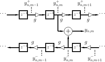
Referring to Fig.C.7, we have the following time-update relations:

\begin{eqnarray*}
y^{+}_{n+1,m}&=& gy^{+}_{n,m-1}\;=\; g\cdot(y_{n,m-1}- y^{-}_{...
..._{n+1,m}&=& gy^{-}_{n,m+1}\;=\; g\cdot(y_{n,m+1}- y^{+}_{n,m+1})
\end{eqnarray*}

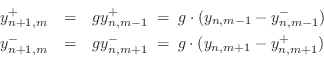
Adding these equations gives

$\displaystyle y_{n+1,m}$ $\displaystyle =$ $\displaystyle g\cdot(y_{n,m-1}+y_{n,m+1})
- g\cdot(\underbrace{y^{-}_{n,m-1}}_{gy^{-}_{n-1,m}} +
\underbrace{y^{+}_{n,m+1}}_{gy^{+}_{n-1,m}})$  
  $\displaystyle =$ $\displaystyle g\cdot(y_{n,m-1}+y_{n,m+1}) - g^2 y_{n-1,m}
\protect$ (C.31)

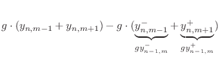
This is now in the form of the finite-difference time-domain (FDTD) scheme analyzed in [222]:

$\displaystyle y_{n+1,m}=
g^{+}_my_{n,m-1}+
g^{-}_my_{n,m+1}+ a_my_{n-1,m},
$

with $ g^{+}_m= g^{-}_m= g$, and $ a_m= -g^2$. In [124], it was shown by von Neumann analysisD.4) that these parameter choices give rise to a stable finite-difference schemeD.2.3), provided $ \vert g\vert\leq 1$. In the present context, we expect stability to follow naturally from starting with a passive digital waveguide model.

Frequency-Dependent Losses

The preceding derivation generalizes immediately to frequency-dependent losses. First imagine each $ g$ in Fig.C.7 to be replaced by $ G(z)$, where for passivity we require

$\displaystyle \left\vert G(e^{j\omega T})\right\vert\leq 1.
$

In the time domain, we interpret $ g(n)$ as the impulse response corresponding to $ G(z)$. We may now derive the frequency-dependent counterpart of Eq.$ \,$(C.31) as follows:

\begin{eqnarray*}
y^{+}_{n+1,m}&=& g\ast y^{+}_{n,m-1}\;=\; g\ast (y_{n,m-1}- y^...
...
&=& g\ast \left[(y_{n,m-1}+y_{n,m+1}) - g\ast y_{n-1,m}\right]
\end{eqnarray*}

where $ \ast $ denotes convolution (in the time dimension only). Define filtered node variables by

\begin{eqnarray*}
y^f_{n,m}&=& g\ast y_{n,m}\\
y^{ff}_{n,m}&=& g\ast y^f_{n,m}.
\end{eqnarray*}

Then the frequency-dependent FDTD scheme is simply

$\displaystyle y_{n+1,m}= y^f_{n,m-1}+ y^f_{n,m+1}- y^{ff}_{n-1,m}.
$

We see that generalizing the FDTD scheme to frequency-dependent losses requires a simple filtering of each node variable $ y_{n,m}$ by the per-sample propagation filter $ G(z)$. For computational efficiency, two spatial lines should be stored in memory at time $ n$: $ y^f_{n,m}$ and $ y^{ff}_{n-1,m}$, for all $ m$. These state variables enable computation of $ y_{n+1,m}$, after which each sample of $ y^f_{n,m}$ ($ \forall m$) is filtered by $ G(z)$ to produce $ y^{ff}_{n-1,m}$ for the next iteration, and $ y_{n+1,m}$ is filtered by $ G(z)$ to produce $ y^f_{n,m}$ for the next iteration.

The frequency-dependent generalization of the FDTD scheme described in this section extends readily to the digital waveguide mesh. See §C.14.5 for the outline of the derivation.


Next Section:
Higher Order Terms
Previous Section:
Digital Filter Models of Damped Strings