


Memoryless Nonlinearities
Memoryless or instantaneous nonlinearities form the simplest and most commonly implemented form of nonlinear element. Furthermore, many complex nonlinear systems can be broken down into a linear system containing a memoryless nonlinearity.
Given a sampled input signal ![]() , the output of any memoryless
nonlinearity can be written as
, the output of any memoryless
nonlinearity can be written as
The fact that a function may be used to describe the nonlinearity implies that each input value is mapped to a unique output value. If it is also true that each output value is mapped to a unique input value, then the function is said to be one-to-one, and the mapping is invertible. If the function is instead ``many-to-one,'' then the inverse is ambiguous, with more than one input value corresponding to the same output value.
Clipping Nonlinearity
A simple example of a noninvertible (many-to-one) memoryless nonlinearity is the clipping nonlinearity, well known to anyone who records or synthesizes audio signals. In normalized form, the clipping nonlinearity is defined by
![$\displaystyle f(x) = \left\{\begin{array}{ll} -1, & x\leq -1 \\ [5pt] x, & -1 \leq x \leq 1 \\ [5pt] 1, & x\geq 1 \\ \end{array} \right. \protect$](http://www.dsprelated.com/josimages_new/pasp/img1514.png)
Since the clipping nonlinearity abruptly transitions from linear to hard-clipped in a non-invertible, heavily aliasing manner, it is usually desirable to use some form of soft-clipping before entering the hard-clipping range.
Arctangent Nonlinearity
A simple example of an invertible (one-to-one) memoryless nonlinearity is the arctangent mapping:
![\includegraphics[width=3in]{eps/atanex}](http://www.dsprelated.com/josimages_new/pasp/img1519.png)
Cubic Soft Clipper
In §9.1.6, we used the cubic soft-clipper to simulate amplifier distortion:
![$\displaystyle f(x) = \left\{\begin{array}{ll}
-\frac{2}{3}, & x\leq -1 \\ [5pt]...
...{3}, & -1 \leq x \leq 1 \\ [5pt]
\frac{2}{3}, & x\geq 1 \\
\end{array}\right.
$](http://www.dsprelated.com/josimages_new/pasp/img1520.png)
![\includegraphics[width=3in]{eps/cnlCopy}](http://www.dsprelated.com/josimages_new/pasp/img1521.png)
Series Expansions
Any ``smooth'' function ![]() can be expanded as a Taylor series expansion:
can be expanded as a Taylor series expansion:
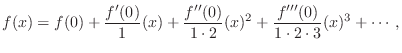
where ``smooth'' means that derivatives of all orders must exist over the range of validity. Derivatives of all orders are obviously needed at
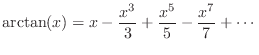
Arctangent Series Expansion
For example, the arctangent function used above can be expanded as
The clipping nonlinearity in Eq.![]() (6.17) is not so amenable to a
series expansion. In fact, it is its own series expansion! Since it
is not differentiable at
(6.17) is not so amenable to a
series expansion. In fact, it is its own series expansion! Since it
is not differentiable at ![]() , it must be represented as three
separate series over the intervals
, it must be represented as three
separate series over the intervals
![]() ,
, ![]() , and
, and
![]() , and the result obtained over these intervals is precisely
the definition of
, and the result obtained over these intervals is precisely
the definition of ![]() in Eq.
in Eq.![]() (6.17).
(6.17).
Spectrum of a Memoryless Nonlinearities
The series expansion of a memoryless nonlinearity is a useful tool for quantifying the aliasing caused by that nonlinear mapping when introduced into the signal path of a discrete-time system.
Square Law Series Expansion
When viewed as a Taylor series expansion such as Eq.![]() (6.18), the
simplest nonlinearity is clearly the square law nonlinearity:
(6.18), the
simplest nonlinearity is clearly the square law nonlinearity:
Consider a simple signal processing system consisting only of the square-law nonlinearity:
Power Law Spectrum
More generally,
In summary, the spectrum at the output of the square-law nonlinearity can be written as
Arctangent Spectrum
Since the series expansion of the arctangent nonlinearity is
Cubic Soft-Clipper Spectrum
The cubic soft-clipper, like any polynomial nonlinearity, is defined directly by its series expansion:
In the absence of hard-clipping (
Stability of Nonlinear Feedback Loops
In general, placing a memoryless nonlinearity ![]() in a stable
feedback loop preserves stability provided the gain of the
nonlinearity is less than one, i.e.,
in a stable
feedback loop preserves stability provided the gain of the
nonlinearity is less than one, i.e.,
![]() . A simple proof
for the case of a loop consisting of a continuous-time delay-line and
memoryless-nonlinearity is as follows.
. A simple proof
for the case of a loop consisting of a continuous-time delay-line and
memoryless-nonlinearity is as follows.
The delay line can be interpreted as a waveguide model of an ideal
string or acoustic pipe having wave impedance ![]() and a noninverting
reflection at its midpoint. A memoryless nonlinearity is a special
case of an arbitrary time-varying gain [449]. By hypothesis,
this gain has magnitude less than one. By routing the output of the
delay line back to its input, the gain plays the role of a reflectance
and a noninverting
reflection at its midpoint. A memoryless nonlinearity is a special
case of an arbitrary time-varying gain [449]. By hypothesis,
this gain has magnitude less than one. By routing the output of the
delay line back to its input, the gain plays the role of a reflectance
![]() at the ``other end'' of the ideal string or acoustic pipe. We can
imagine, for example, a terminating dashpot with randomly varying
positive resistance
at the ``other end'' of the ideal string or acoustic pipe. We can
imagine, for example, a terminating dashpot with randomly varying
positive resistance ![]() . The set of all
. The set of all ![]() corresponds to
the set of real reflection coefficients
corresponds to
the set of real reflection coefficients
![]() in the
open interval
in the
open interval ![]() . Thus, each instantaneous nonlinearity-gain
. Thus, each instantaneous nonlinearity-gain
![]() corresponds to some instantaneously positive resistance
corresponds to some instantaneously positive resistance
![]() . The whole system is therefore passive, even as
. The whole system is therefore passive, even as ![]() changes arbitrarily (while remaining positive). (It is perhaps easier
to ponder a charged capacitor
changes arbitrarily (while remaining positive). (It is perhaps easier
to ponder a charged capacitor ![]() terminated on a randomly varying
resistor
terminated on a randomly varying
resistor ![]() .) This proof method immediately extends to nonlinear
feedback around any transfer function that can be interpreted as the
reflectance of a passive physical system, i.e., any transfer function
.) This proof method immediately extends to nonlinear
feedback around any transfer function that can be interpreted as the
reflectance of a passive physical system, i.e., any transfer function
![]() for which the gain is bounded by 1 at each frequency, viz.,
for which the gain is bounded by 1 at each frequency, viz.,
![]() .
.
The finite-sampling-rate case can be embedded in a passive
infinite-sampling-rate case by replacing each sample with a constant
pulse lasting ![]() seconds (in the delay line).
The continuous-time memoryless nonlinearity
seconds (in the delay line).
The continuous-time memoryless nonlinearity ![]() is similarly a
held version of the discrete-time case
is similarly a
held version of the discrete-time case ![]() . Since the
discrete-time case is a simple sampling of the (passive)
continuous-time case, we are done.
. Since the
discrete-time case is a simple sampling of the (passive)
continuous-time case, we are done.
Practical Advice
In summary, the following pointers can be offered regarding nonlinear elements in a digital waveguide model:
- Verify that aliasing can be heard and sounds bad before working
to get rid of it.
- Aliasing (bandwidth expansion) is reduced by smoothing
``corners'' in the nonlinearity.
- Consider an oversampling factor for nonlinear
subsystems sufficient to accommodate the bandwidth expansion
caused by the nonlinearity.
- Make sure there is adequate lowpass filtering in a feedback loop
containing a nonlinearity.
 oversampling, and
- a lowpass filter to
![$ \omega\in[-\pi/3,\pi/3]$](http://www.dsprelated.com/josimages_new/pasp/img1557.png) after the nonlinearity.
after the nonlinearity.
Another variation is to oversample by two, in which case there is aliasing, but that aliasing does not reach the ``base band.'' Therefore, a half-band lowpass filter rejects both the second spectral image and the third, which is aliased onto the second.
Next Section:
Dashpot
Previous Section:
Longitudinal Waves


