


Numerical Integration of General State-Space Models
An approximate discrete-time numerical solution of Eq.![]() (1.6) is provided by
(1.6) is provided by
Let
This is a simple example of numerical integration for solving
an ODE, where in this case the ODE is given by Eq.![]() (1.6) (a very
general, potentially nonlinear, vector ODE). Note that the initial
state
(1.6) (a very
general, potentially nonlinear, vector ODE). Note that the initial
state
![]() is required to start Eq.
is required to start Eq.![]() (1.7) at time zero;
the initial state thus provides boundary conditions for the ODE at
time zero. The time sampling interval
(1.7) at time zero;
the initial state thus provides boundary conditions for the ODE at
time zero. The time sampling interval ![]() may be fixed for all
time as
may be fixed for all
time as ![]() (as it normally is in linear, time-invariant
digital signal processing systems), or it may vary adaptively
according to how fast the system is changing (as is often needed for
nonlinear and/or time-varying systems). Further discussion of
nonlinear ODE solvers is taken up in §7.4, but for most of
this book, linear, time-invariant systems will be emphasized.
(as it normally is in linear, time-invariant
digital signal processing systems), or it may vary adaptively
according to how fast the system is changing (as is often needed for
nonlinear and/or time-varying systems). Further discussion of
nonlinear ODE solvers is taken up in §7.4, but for most of
this book, linear, time-invariant systems will be emphasized.
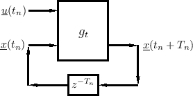
Note that for handling switching states (such as op-amp
comparators and the like), the discrete-time state-space formulation
of Eq.![]() (1.7) is more conveniently applicable than the
continuous-time formulation in Eq.
(1.7) is more conveniently applicable than the
continuous-time formulation in Eq.![]() (1.6).
(1.6).
Next Section:
State Definition
Previous Section:
State-Space Model of a Force-Driven Mass


