


Physical Digital Filters
Analog Computers
Analog filters are inherently ``physical'' since voltages and currents are direct ``analogs'' for physical variables such as force and velocity. So-called ``analog computers'' were often used for physical system simulation before digital computers took over.
Finite Difference Methods
One of the first applications of digital computers to numerical
simulation of physical systems was the so-called finite
difference approach [481].
The general
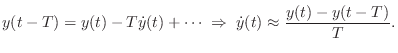
procedure is to replace derivatives by finite differences, and there
are many variations on how this can be done. For example, the first
partial derivative with respect to time in Eq.![]() (A.1) may be
approximated by
(A.1) may be
approximated by
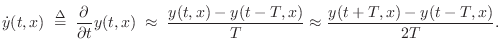
The second form, called a centered finite difference, has the advantage of not introducing a time delay, but at the expense of requiring an extra factor of two oversampling for a given accuracy in its magnitude response (when viewed as a digital filter).
Finite differences are at least as old as Taylor series, since,
Interestingly, the general Taylor series, published in 1715 by Taylor in his book Methodus Incrementorum Directa et Inversa, was known more than forty years earlier to James Gregory (1668), somewhat earlier to Jean Bernoulli, and to some extent even before 1550 in India [65, pp. 422,469].
Finite differences were used to construct the earliest known digital models of vibrating strings by Pierre Ruiz and Lejaren Hiller ca. 1971 [194].
Finite-difference methods have not historically been aimed at real-time simulation, and they are generally used with very large sampling rates compared with the ``band of interest''. On the order of ten-times oversampling is needed to obtain reasonably accurate simulation across the entire audio band when using classical finite difference methods. In the finite-difference method literature, accuracy is usually only considered at dc, which is inaudible. Since finite difference models are usually linear, time-invariant digital filters, it is straightforward to improve them by filter-design methods, optimizing perceived audio error over the entire audio band. Such improved (and optionally extended) coefficients can then be used to construct a refined, indirectly estimated, partial differential equation.
Other offline (slower than real time) computational physical modeling methods include finite element [480] and boundary element methods. Such offline simulations can be valuable as a source of ``virtual experiments'' which enable the testing and calibration of faster algorithms. As an example, a detailed simulation of guitar acoustics, employing both finite difference and finite element modeling approaches, is reported in [109].
Transfer Function Models
As indicated in the previous section, instead of digitizing a differential equation by finite differences, one can often formulate a filter design problem. This is ideal when all that matters is the input-output response of the physical system, and the physical system is linear and time-invariant (LTI). When the desired transfer function spans more than one system element, non-physical models are usually obtained, so we will not consider such models further. However, digital filter design methods optimizing perceptually motivated error criteria are extremely effective in spectral modeling and audio compression applications [337]. They are also good choices for subsystems which are to remain fixed over time, such as cello bodies, piano soundboards, and the like.
Wave Digital Filter Models
Perhaps the best known physics-based approach to digital filter design is wave digital filters, developed principally by Alfred Fettweis [136].A.9Wave digital filters may be constructed by applying the bilinear transform [343] to the scattering-theoretic formulation of lumped RLC networks introduced in circuit theory by Vitold Belevitch [34]. Fettweis in fact worked with Belevitch.A.10Scattering theory had been in use for many years prior in quantum mechanics.
A key, driving property of wave digital filters is low sensitivity to coefficient round-off error. This follows from the correspondence to passive circuit networks. Wave digital filters also have the nice property of preserving order of the original (analog) system. For example, a ``wave digital spring'' is simply a unit delay, and a ``wave digital mass'' is a unit delay with a sign flip. The only approximation aspect is the frequency-warping caused by the bilinear transform. It is interesting to note that when it is possible to frequency-warp input/output signals exactly, a wave digital filter can implement a continuous-time LTI system exactly! See [55] for a discussion of wave digital filters and their relation to finite differences et al.
In computer music, various ``wave digital elements'' have been proposed, including wave digital toneholes [527], piano hammers [56], and woodwind bores [525].
Next Section:
Voice Synthesis
Previous Section:
Sampling Theory


