


Physical Models
We now turn to the main subject of this book, physical models of musical instruments and audio effects. In contrast to the non-physical signal models mentioned above, we will consider a signal model to be a physical signal model when there is an explicit representation of the relevant physical state of the sound source. For example, a string physical model must offer the possibility of exciting the string at any point along its length.
We begin with a review of physical models in general, followed by an overview of computational subtypes, with some indication of their relative merits, and what is and is not addressed in this book.
All We Need is Newton
Since there are no relativistic or quantum effects to worry about in musical instruments or audio effects (at least not yet), good old Newtonian mechanics will suffice for our purposes. Newton's three laws of motion can be summarized by the classic equation2.4
However, the apparent mathematical simplicity of Newton's basic laws of motion does not mean that our task will always be easy. Models based on Newton's laws can quickly become prohibitively complex. We will usually need many further simplifications that preserve both sound quality and expressivity of control.
Formulations
Below are various physical-model representations we will consider:
- Ordinary Differential Equations (ODE)
- Partial Differential Equations (PDE)
- Difference Equations (DE)
- Finite Difference Schemes (FDS)
- (Physical) State Space Models
- Transfer Functions (between physical signals)
- Modal Representations (Parallel Second-Order Filter Sections)
- Equivalent Circuits
- Impedance Networks
- Wave Digital Filters (WDF)
- Digital Waveguide (DW) Networks
ODEs and PDEs are purely mathematical descriptions (being differential equations), but they can be readily ``digitized'' to obtain computational physical models.2.5Difference equations are simply digitized differential equations. That is, digitizing ODEs and PDEs produces DEs. A DE may also be called a finite difference scheme. A discrete-time state-space model is a special formulation of a DE in which a vector of state variables is defined and propagated in a systematic way (as a vector first-order finite-difference scheme). A linear difference equation with constant coefficients--the Linear, Time-Invariant (LTI) case--can be reduced to a collection of transfer functions, one for each pairing of input and output signals (or a single transfer function matrix can relate a vector of input signal z transforms to a vector of output signal z transforms). An LTI state-space model can be diagonalized to produce a so-called modal representation, yielding a computational model consisting of a parallel bank of second-order digital filters. Impedance networks and their associated equivalent circuits are at the foundations of electrical engineering, and analog circuits have been used extensively to model linear systems and provide many useful functions. They are also useful intermediate representations for developing computational physical models in audio. Wave Digital Filters (WDF) were introduced as a means of digitizing analog circuits element by element, while preserving the ``topology'' of the original analog circuit (a very useful property when parameters are time varying as they often are in audio effects). Digital waveguide networks can be viewed as highly efficient computational forms for propagating solutions to PDEs allowing wave propagation. They can also be used to ``compress'' the computation associated with a sum of quasi harmonically tuned second-order resonators.
All of the above techniques are discussed to varying extents in this book. The following sections provide a bit more introduction before plunging into the chapters that follow.
ODEs
Ordinary Differential Equations (ODEs) typically result directly from Newton's laws of motion, restated here as follows:
This is a second-order ODE relating the force
If the applied force ![]() is due to a spring with spring-constant
is due to a spring with spring-constant
![]() , then we may write the ODE as
, then we may write the ODE as
If the mass is sliding with friction, then a simple ODE model is given by
We will use such ODEs to model mass, spring, and dashpot2.6 elements in Chapter 7.
PDEs
A partial differential equation (PDE) extends ODEs by adding
one or more independent variables (usually spatial variables). For
example, the wave equation for the ideal vibrating string adds one
spatial dimension ![]() (along the axis of the string) and may be written as
follows:
(along the axis of the string) and may be written as
follows:
| (2.1) |
where
Difference Equations (Finite Difference Schemes)
There are many methods for converting ODEs and PDEs to difference equations [53,55,481]. As will be discussed in §7.3, a very simple, order-preserving method is to replace each derivative with a finite difference:
![$\displaystyle \dot x(t)\isdefs \frac{d}{dt} x(t) \isdefs \lim_{\delta\to 0} \frac{x(t) - x(t-\delta)}{\delta} \;\approx\; \frac{x(n T)-x[(n-1)T]}{T} \protect$](http://www.dsprelated.com/josimages_new/pasp/img187.png)
for sufficiently small
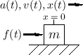
As a simple example, consider a mass ![]() driven along a frictionless
surface by a driving force
driven along a frictionless
surface by a driving force ![]() , as in Fig.1.1, and
suppose we wish to know the resulting velocity of the mass
, as in Fig.1.1, and
suppose we wish to know the resulting velocity of the mass ![]() ,
assuming it starts out with position and velocity 0 at time 0
(i.e.,
,
assuming it starts out with position and velocity 0 at time 0
(i.e.,
![]() ). Then, from Newton's
). Then, from Newton's ![]() relation, the ODE is
relation, the ODE is
![$\displaystyle f(nT) \eqsp m \frac{v(nT) - v[(n-1)T]}{T}, \quad n=0,1,2,\ldots\,.
$](http://www.dsprelated.com/josimages_new/pasp/img191.png)
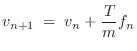
![$\displaystyle v(nT) \eqsp v[(n-1)T] + \frac{T}{m} f(nT), \quad n=0,1,2,\ldots \protect$](http://www.dsprelated.com/josimages_new/pasp/img193.png)
with
![$\displaystyle \dot x(t) \eqsp \lim_{\delta\to 0} \frac{x(t+\delta) - x(t)}{\delta} \;\approx\; \frac{x[(n+1)T]-x(n T)}{T} \protect$](http://www.dsprelated.com/josimages_new/pasp/img198.png)
As
![$\displaystyle v[(n+1)T] \eqsp v(nT) + \frac{T}{m} f(nT), \quad n=0,1,2,\ldots \protect$](http://www.dsprelated.com/josimages_new/pasp/img200.png)
with
A finite difference scheme is said to be explicit when it can be computed forward in time in terms of quantities from previous time steps, as in this example. Thus, an explicit finite difference scheme can be implemented in real time as a causal digital filter.
There are also implicit finite-difference schemes which may correspond to non-causal digital filters [449]. Implicit schemes are generally solved using iterative and/or matrix-inverse methods, and they are typically used offline (not in real time) [555].
There is also an interesting class of explicit schemes called semi-implicit finite-difference schemes which are obtained from an implicit scheme by imposing a fixed upper limit on the number of iterations in, say, Newton's method for iterative solution [555]. Thus, any implicit scheme that can be quickly solved by iterative methods can be converted to an explicit scheme for real-time usage. One technique for improving the iterative convergence rate is to work at a very high sampling rate, and initialize the iteration for each sample at the solution for the previous sample [555].
In this book, we will be concerned almost exclusively with explicit linear finite-difference schemes, i.e., causal digital filter models of one sort or another. That is, the main thrust is to obtain as much ``physical modeling power'' as possible from ordinary digital filters and delay lines. We will also be able to easily add memoryless nonlinearities where needed (such as implemented by table look-ups and short polynomial evaluations) as a direct result of the physical meaning of the signal samples.
State Space Models
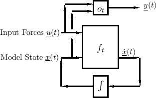
Equations of motion for any physical system may be conveniently formulated in terms of the state of the system [330]:
Here,
Equation (1.6) is diagrammed in Fig.1.4.
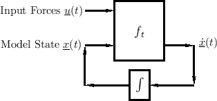
The key property of the state vector
![]() in this formulation is
that it completely determines the system at time
in this formulation is
that it completely determines the system at time ![]() , so that
future states depend only on the current state and on any inputs at
time
, so that
future states depend only on the current state and on any inputs at
time ![]() and beyond.2.8 In particular, all past states and the
entire input history are ``summarized'' by the current state
and beyond.2.8 In particular, all past states and the
entire input history are ``summarized'' by the current state
![]() .
Thus,
.
Thus,
![]() must include all ``memory'' of the system.
must include all ``memory'' of the system.
Forming Outputs
Any system output is some function of the state, and possibly the input (directly):
The general case of output extraction is shown in Fig.1.5.
The output signal (vector) is most typically a linear combination of state variables and possibly the current input:
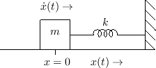
State-Space Model of a Force-Driven Mass
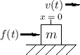
For the simple example of a mass ![]() driven by external force
driven by external force ![]() along the
along the ![]() axis, we have the system of Fig.1.6.
We should choose the state variable to be velocity
axis, we have the system of Fig.1.6.
We should choose the state variable to be velocity
![]() so that
Newton's
so that
Newton's ![]() yields
yields
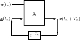
Numerical Integration of General State-Space Models
An approximate discrete-time numerical solution of Eq.![]() (1.6) is provided by
(1.6) is provided by
Let
This is a simple example of numerical integration for solving
an ODE, where in this case the ODE is given by Eq.![]() (1.6) (a very
general, potentially nonlinear, vector ODE). Note that the initial
state
(1.6) (a very
general, potentially nonlinear, vector ODE). Note that the initial
state
![]() is required to start Eq.
is required to start Eq.![]() (1.7) at time zero;
the initial state thus provides boundary conditions for the ODE at
time zero. The time sampling interval
(1.7) at time zero;
the initial state thus provides boundary conditions for the ODE at
time zero. The time sampling interval ![]() may be fixed for all
time as
may be fixed for all
time as ![]() (as it normally is in linear, time-invariant
digital signal processing systems), or it may vary adaptively
according to how fast the system is changing (as is often needed for
nonlinear and/or time-varying systems). Further discussion of
nonlinear ODE solvers is taken up in §7.4, but for most of
this book, linear, time-invariant systems will be emphasized.
(as it normally is in linear, time-invariant
digital signal processing systems), or it may vary adaptively
according to how fast the system is changing (as is often needed for
nonlinear and/or time-varying systems). Further discussion of
nonlinear ODE solvers is taken up in §7.4, but for most of
this book, linear, time-invariant systems will be emphasized.
Note that for handling switching states (such as op-amp
comparators and the like), the discrete-time state-space formulation
of Eq.![]() (1.7) is more conveniently applicable than the
continuous-time formulation in Eq.
(1.7) is more conveniently applicable than the
continuous-time formulation in Eq.![]() (1.6).
(1.6).
State Definition
In view of the above discussion, it is perhaps plausible that the
state
![]() of a physical
system at time
of a physical
system at time ![]() can be defined as a collection of state
variables
can be defined as a collection of state
variables ![]() , wherein each state variable
, wherein each state variable ![]() is a
physical amplitude (pressure, velocity, position,
is a
physical amplitude (pressure, velocity, position, ![]() )
corresponding to a degree of freedom of the system. We define a
degree of freedom as a single dimension of energy
storage. The net result is that it is possible to compute the
stored energy in any degree of freedom (the system's ``memory'') from
its corresponding state-variable amplitude.
)
corresponding to a degree of freedom of the system. We define a
degree of freedom as a single dimension of energy
storage. The net result is that it is possible to compute the
stored energy in any degree of freedom (the system's ``memory'') from
its corresponding state-variable amplitude.
For example, an ideal mass ![]() can store only kinetic
energy
can store only kinetic
energy
![]() , where
, where
![]() denotes the
mass's velocity along the
denotes the
mass's velocity along the ![]() axis. Therefore, velocity is the
natural choice of state variable for an ideal point-mass.
Coincidentally, we reached this conclusion independently above by
writing
axis. Therefore, velocity is the
natural choice of state variable for an ideal point-mass.
Coincidentally, we reached this conclusion independently above by
writing ![]() in state-space form
in state-space form
![]() . Note that a
point mass that can move freely in 3D space has three degrees of
freedom and therefore needs three state variables
. Note that a
point mass that can move freely in 3D space has three degrees of
freedom and therefore needs three state variables
![]() in
its physical model. In typical models from musical acoustics (e.g.,
for the piano hammer), masses are allowed only one degree of freedom,
corresponding to being constrained to move along a 1D line, like an
ideal spring. We'll study the ideal mass further in §7.1.2.
in
its physical model. In typical models from musical acoustics (e.g.,
for the piano hammer), masses are allowed only one degree of freedom,
corresponding to being constrained to move along a 1D line, like an
ideal spring. We'll study the ideal mass further in §7.1.2.
Another state-variable example is provided by an ideal spring
described by Hooke's law ![]() (§B.1.3), where
(§B.1.3), where ![]() denotes the spring
constant, and
denotes the spring
constant, and ![]() denotes the spring displacement from rest. Springs
thus contribute a force proportional to displacement in Newtonian
ODEs. Such a spring can only store the physical work (force
times distance), expended to displace, it in the form of
potential energy
denotes the spring displacement from rest. Springs
thus contribute a force proportional to displacement in Newtonian
ODEs. Such a spring can only store the physical work (force
times distance), expended to displace, it in the form of
potential energy
![]() . More about
ideal springs will be discussed in §7.1.3. Thus,
spring displacement is the most natural choice of state
variable for a spring.
. More about
ideal springs will be discussed in §7.1.3. Thus,
spring displacement is the most natural choice of state
variable for a spring.
In so-called RLC electrical circuits (consisting of resistors ![]() ,
inductors
,
inductors ![]() , and capacitors
, and capacitors ![]() ), the state variables are
typically defined as all of the capacitor voltages (or charges) and
inductor currents. We will discuss RLC electrical circuits further
below.
), the state variables are
typically defined as all of the capacitor voltages (or charges) and
inductor currents. We will discuss RLC electrical circuits further
below.
There is no state variable for each resistor current in an RLC circuit
because a resistor dissipates energy but does not store it--it has no
``memory'' like capacitors and inductors. The state (current ![]() ,
say) of a resistor
,
say) of a resistor ![]() is determined by the voltage
is determined by the voltage ![]() across it,
according to Ohm's law
across it,
according to Ohm's law ![]() , and that voltage is supplied by the
capacitors, inductors, and voltage-sources, etc., to which it is
connected. Analogous remarks apply to the dashpot, which is
the mechanical analog of the resistor--we do not assign state
variables to dashpots. (If we do, such as by mistake, then we will
obtain state variables that are linearly dependent on other state
variables, and the order of the system appears to be larger than it
really is. This does not normally cause problems, and there are many
numerical ways to later ``prune'' the state down to its proper order.)
, and that voltage is supplied by the
capacitors, inductors, and voltage-sources, etc., to which it is
connected. Analogous remarks apply to the dashpot, which is
the mechanical analog of the resistor--we do not assign state
variables to dashpots. (If we do, such as by mistake, then we will
obtain state variables that are linearly dependent on other state
variables, and the order of the system appears to be larger than it
really is. This does not normally cause problems, and there are many
numerical ways to later ``prune'' the state down to its proper order.)
Masses, springs, dashpots, inductors, capacitors, and resistors are examples of so-called lumped elements. Perhaps the simplest distributed element is the continuous ideal delay line. Because it carries a continuum of independent amplitudes, the order (number of state variables) is infinity for a continuous delay line of any length! However, in practice, we often work with sampled, bandlimited systems, and in this domain, delay lines have a finite number of state variables (one for each delay element). Networks of lumped elements yield finite-order state-space models, while even one distributed element jumps the order to infinity until it is bandlimited and sampled.
In summary, a state variable may be defined as a physical amplitude for some energy-storing degree of freedom. In models of mechanical systems, a state variable is needed for each ideal spring and point mass (times the number of dimensions in which it can move). For RLC electric circuits, a state variable is needed for each capacitor and inductor. If there are any switches, their state is also needed in the state vector (e.g., as boolean variables). In discrete-time systems such as digital filters, each unit-sample delay element contributes one (continuous) state variable to the model.
Linear State Space Models
As introduced in Book II [449, Appendix G], in the linear,
time-invariant case, a discrete-time state-space model looks
like a vector first-order finite-difference model:
where
The state-space representation is especially powerful for
multi-input, multi-output (MIMO) linear systems, and also for
time-varying linear systems (in which case any or all of the
matrices in Eq.![]() (1.8) may have time subscripts
(1.8) may have time subscripts ![]() ) [220].
) [220].
To cast the previous force-driven mass example in state-space form, we
may first observe that the state of the mass is specified by its
velocity ![]() and position
and position
![]() , or
, or
![]() .2.9Thus, to Eq.
.2.9Thus, to Eq.![]() (1.5) we may add the explicit difference equation
(1.5) we may add the explicit difference equation
![$\displaystyle x[(n+1)T] \eqsp x(nT) + T\,v(nT)
\eqsp x(nT) + T\,v[(n-1)T] + \frac{T^2}{m} f[(n-1)T]
$](http://www.dsprelated.com/josimages_new/pasp/img255.png)
![$\displaystyle \left[\begin{array}{c} x_{n+1} \\ [2pt] v_{n+1} \end{array}\right...
...ray}{c} 0 \\ [2pt] T/m \end{array}\right] f_n, \quad n=0,1,2,\ldots\,, \protect$](http://www.dsprelated.com/josimages_new/pasp/img257.png)
with
General features of this example are that the entire physical state of
the system is collected together into a single vector, and the
elements of the ![]() matrices include physical parameters (and
the sampling interval, in the discrete-time case). The parameters may
also vary with time (time-varying systems), or be functions of the
state (nonlinear systems).
matrices include physical parameters (and
the sampling interval, in the discrete-time case). The parameters may
also vary with time (time-varying systems), or be functions of the
state (nonlinear systems).
The general procedure for building a state-space model is to label all
the state variables and collect them into a vector
![]() , and then
work out the state-transition matrix
, and then
work out the state-transition matrix ![]() , input gains
, input gains ![]() , output
gains
, output
gains ![]() , and any direct coefficient
, and any direct coefficient ![]() . A state variable
. A state variable
![]() is needed for each lumped energy-storage element (mass,
spring, capacitor, inductor), and one for each sample of delay in
sampled distributed systems. After that, various equivalent (but
numerically preferable) forms can be generated by means of
similarity transformations [449, pp. 360-374]. We
will make sparing use of state-space models in this book, because
they can be linear-algebra intensive, and therefore rarely used in
practical real-time signal processing systems for music and audio
effects. However, the state-space framework is an important
general-purpose tool that should be kept in mind [220], and
there is extensive support for state-space models in the matlab
(``matrix laboratory'') language and its libraries. We will use it
mainly as an analytical tool from time to time.
is needed for each lumped energy-storage element (mass,
spring, capacitor, inductor), and one for each sample of delay in
sampled distributed systems. After that, various equivalent (but
numerically preferable) forms can be generated by means of
similarity transformations [449, pp. 360-374]. We
will make sparing use of state-space models in this book, because
they can be linear-algebra intensive, and therefore rarely used in
practical real-time signal processing systems for music and audio
effects. However, the state-space framework is an important
general-purpose tool that should be kept in mind [220], and
there is extensive support for state-space models in the matlab
(``matrix laboratory'') language and its libraries. We will use it
mainly as an analytical tool from time to time.
As noted earlier, a point mass only requires a first-order model:
Impulse Response of State Space Models
As derived in Book II [449, Appendix G], the impulse response of the state-space model can be summarized as
![$\displaystyle {\mathbf{h}}(n) \eqsp \left\{\begin{array}{ll} D, & n=0 \\ [5pt] CA^{n-1}B, & n>0 \\ \end{array} \right. \protect$](http://www.dsprelated.com/josimages_new/pasp/img268.png)
Thus, the
In our force-driven-mass example, we have ![]() ,
,
![]() , and
, and
![]() . For a position output we have
. For a position output we have ![]() while for a velocity
output we would set
while for a velocity
output we would set ![]() . Choosing
. Choosing
![]() simply feeds
the whole state vector to the output, which allows us to look at both
simultaneously:
simply feeds
the whole state vector to the output, which allows us to look at both
simultaneously:
![\begin{eqnarray*}
{\mathbf{h}}(n+1) &=&\left[\begin{array}{cc} 1 & 0 \\ [2pt] 0 ...
...\left[\begin{array}{c} nT \\ [2pt] 1 \end{array}\right]
\protect
\end{eqnarray*}](http://www.dsprelated.com/josimages_new/pasp/img278.png)
Thus, when the input force is a unit pulse, which corresponds
physically to imparting momentum ![]() at time 0 (because the
time-integral of force is momentum and the physical area under a unit
sample is the sampling interval
at time 0 (because the
time-integral of force is momentum and the physical area under a unit
sample is the sampling interval ![]() ), we see that the velocity after
time 0 is a constant
), we see that the velocity after
time 0 is a constant ![]() , or
, or ![]() , as expected from
conservation of momentum. If the velocity is constant, then the
position must grow linearly, as we see that it does:
, as expected from
conservation of momentum. If the velocity is constant, then the
position must grow linearly, as we see that it does:
![]() . The finite difference approximation to the time-derivative
of
. The finite difference approximation to the time-derivative
of ![]() now gives
now gives
![]() , for
, for ![]() , which
is consistent.
, which
is consistent.
Zero-Input Response of State Space Models
The response of a state-space model Eq.![]() (1.8) to initial
conditions, i.e., its initial state
(1.8) to initial
conditions, i.e., its initial state
![]() , is given by
, is given by
In our force-driven mass example, with the external force set to zero,
we have, from Eq.![]() (1.9) or Eq.
(1.9) or Eq.![]() (1.11),
(1.11),
![$\displaystyle \left[\begin{array}{c} x_{n+1} \\ [2pt] v_{n+1} \end{array}\right...
...ght]
\eqsp \left[\begin{array}{c} x_0+v_0 n T \\ [2pt] v_0 \end{array}\right].
$](http://www.dsprelated.com/josimages_new/pasp/img286.png)
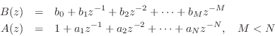
Transfer Functions
As developed in Book II [449], a discrete-time transfer function is the z transform of the impulse response of a linear, time-invariant (LTI) system. In a physical modeling context, we must specify the input and output signals we mean for each transfer function to be associated with the LTI model. For example, if the system is a simple mass sliding on a surface, the input signal could be an external applied force, and the output could be the velocity of the mass in the direction of the applied force. In systems containing many masses and other elements, there are many possible different input and output signals. It is worth emphasizing that a system can be reduced to a set of transfer functions only in the LTI case, or when the physical system is at least nearly linear and only slowly time-varying (compared with its impulse-response duration).
As we saw in the previous section, the state-space formulation nicely
organizes all possible input and output signals in a linear system.
Specifically, for inputs, each input signal is multiplied by a ``![]() vector'' (the corresponding column of the
vector'' (the corresponding column of the ![]() matrix) and added to the
state vector; that is, each input signal may be arbitrarily scaled and
added to any state variable. Similarly, each state variable may be
arbitrarily scaled and added to each output signal via the row of the
matrix) and added to the
state vector; that is, each input signal may be arbitrarily scaled and
added to any state variable. Similarly, each state variable may be
arbitrarily scaled and added to each output signal via the row of the
![]() matrix corresponding to that output signal.
matrix corresponding to that output signal.
Using the closed-form sum of a matrix geometric series (again as
detailed in Book II), we may easily calculate the transfer function of
the state-space model of Eq.![]() (1.8) above as the z transform of the
impulse response given in Eq.
(1.8) above as the z transform of the
impulse response given in Eq.![]() (1.10) above:
(1.10) above:
Note that if there are
In the force-driven-mass example of the previous section, defining the
input signal as the driving force ![]() and the output signal as the
mass velocity
and the output signal as the
mass velocity ![]() , we have
, we have ![]() ,
,
![]() ,
, ![]() ,
and
,
and ![]() , so that the force-to-velocity transfer function is given by
, so that the force-to-velocity transfer function is given by
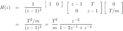
![\begin{eqnarray*}
H(z)
&=& D + C \left(zI - A\right)^{-1}B\\ [5pt]
&=&\begin{ar...
...{z-1}{(z-1)^2} \eqsp \zbox {\frac{T}{m}\frac{z^{-1}}{1-z^{-1}}.}
\end{eqnarray*}](http://www.dsprelated.com/josimages_new/pasp/img293.png)
Thus, the force-to-velocity transfer function is a one-pole filter
with its pole at ![]() (an integrator). The unit-sample delay in the
numerator guards against delay-free loops when this element (a mass)
is combined with other elements to build larger filter structures.
(an integrator). The unit-sample delay in the
numerator guards against delay-free loops when this element (a mass)
is combined with other elements to build larger filter structures.
Similarly, the force-to-position transfer function is a two-pole filter:
Now we have two poles on the unit circle at ![]() , and the impulse
response of this filter is a ramp, as already discovered from the
previous impulse-response calculation.
, and the impulse
response of this filter is a ramp, as already discovered from the
previous impulse-response calculation.
Once we have transfer-function coefficients, we can realize any of a large number of digital filter types, as detailed in Book II [449, Chapter 9].
Modal Representation
One of the filter structures introduced in Book II [449, p.
209] was the parallel second-order filter bank, which
may be computed from the general transfer function (a ratio of
polynomials in ![]() ) by means of the Partial Fraction Expansion
(PFE) [449, p. 129]:
) by means of the Partial Fraction Expansion
(PFE) [449, p. 129]:
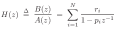
where
The PFE Eq.![]() (1.12) expands the (strictly proper2.10) transfer function as a
parallel bank of (complex) first-order resonators. When the
polynomial coefficients
(1.12) expands the (strictly proper2.10) transfer function as a
parallel bank of (complex) first-order resonators. When the
polynomial coefficients ![]() and
and ![]() are real, complex poles
are real, complex poles ![]() and
residues
and
residues ![]() occur in conjugate pairs, and these can be
combined to form second-order sections [449, p. 131]:
occur in conjugate pairs, and these can be
combined to form second-order sections [449, p. 131]:
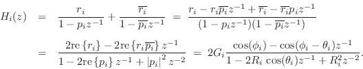
where
![]() and
and
![]() . Thus, every transfer function
. Thus, every transfer function ![]() with real
coefficients can be realized as a parallel bank of real first- and/or
second-order digital filter sections, as well as a parallel FIR branch
when
with real
coefficients can be realized as a parallel bank of real first- and/or
second-order digital filter sections, as well as a parallel FIR branch
when ![]() .
.
As we will develop in §8.5, modal synthesis employs a ``source-filter'' synthesis model consisting of some driving signal into a parallel filter bank in which each filter section implements the transfer function of some resonant mode in the physical system. Normally each section is second-order, but it is sometimes convenient to use larger-order sections; for example, fourth-order sections have been used to model piano partials in order to have beating and two-stage-decay effects built into each partial individually [30,29].
For example, if the physical system were a row of tuning forks (which are designed to have only one significant resonant frequency), each tuning fork would be represented by a single (real) second-order filter section in the sum. In a modal vibrating string model, each second-order filter implements one ``ringing partial overtone'' in response to an excitation such as a finger-pluck or piano-hammer-strike.
State Space to Modal Synthesis
The partial fraction expansion works well to create a modal-synthesis system from a transfer function. However, this approach can yield inefficient realizations when the system has multiple inputs and outputs, because in that case, each element of the transfer-function matrix must be separately expanded by the PFE. (The poles are the same for each element, unless they are canceled by zeros, so it is really only the residue calculations that must be carried out for each element.)
If the second-order filter sections are realized in direct-form-II or transposed-direct-form-I (or more generally in any form for which the poles effectively precede the zeros), then the poles can be shared among all the outputs for each input, since the poles section of the filter from that input to each output sees the same input signal as all others, resulting in the same filter state. Similarly, the recursive portion can be shared across all inputs for each output when the filter sections have poles implemented after the zeros in series; one can imagine ``pushing'' the identical two-pole filters through the summer used to form the output signal. In summary, when the number of inputs exceeds the number of outputs, the poles are more efficiently implemented before the zeros and shared across all outputs for each input, and vice versa. This paragraph can be summarized symbolically by the following matrix equation:
![$\displaystyle \left[\begin{array}{c} y_1 \\ [2pt] y_2 \end{array}\right]
\eqsp...
...{\frac{1}{A}\left[\begin{array}{c} u_1 \\ [2pt] u_2 \end{array}\right]\right\}
$](http://www.dsprelated.com/josimages_new/pasp/img306.png)
What may not be obvious when working with transfer functions alone is
that it is possible to share the poles across all of the inputs
and outputs! The answer? Just diagonalize a state-space
model by means of a similarity transformation [449, p.
360]. This will be discussed a bit further in
§8.5. In a diagonalized state-space model, the ![]() matrix is diagonal.2.11 The
matrix is diagonal.2.11 The ![]() matrix provides
routing and scaling for all the input signals driving the modes. The
matrix provides
routing and scaling for all the input signals driving the modes. The
![]() matrix forms the appropriate linear combination of modes for each
output signal. If the original state-space model is a physical model,
then the transformed system gives a parallel filter bank that is
excited from the inputs and observed at the outputs in a physically
correct way.
matrix forms the appropriate linear combination of modes for each
output signal. If the original state-space model is a physical model,
then the transformed system gives a parallel filter bank that is
excited from the inputs and observed at the outputs in a physically
correct way.
Force-Driven-Mass Diagonalization Example
To diagonalize our force-driven mass example, we may begin with its
state-space model Eq.![]() (1.9):
(1.9):
![$\displaystyle \left[\begin{array}{c} x_{n+1} \\ [2pt] v_{n+1} \end{array}\right...
...t[\begin{array}{c} 0 \\ [2pt] T/m \end{array}\right] f_n, \quad n=0,1,2,\ldots
$](http://www.dsprelated.com/josimages_new/pasp/img307.png)
Typical State-Space Diagonalization Procedure
As discussed in [449, p. 362] and exemplified in
§C.17.6, to diagonalize a system, we must find the
eigenvectors of ![]() by solving
by solving
| (2.13) |
where
The transformed system describes the same system as in Eq.
Efficiency of Diagonalized State-Space Models
Note that a general ![]() th-order state-space model Eq.
th-order state-space model Eq.![]() (1.8) requires
around
(1.8) requires
around ![]() multiply-adds to update for each time step (assuming the
number of inputs and outputs is small compared with the number of
state variables, in which case the
multiply-adds to update for each time step (assuming the
number of inputs and outputs is small compared with the number of
state variables, in which case the
![]() computation dominates).
After diagonalization by a similarity transform, the time update is
only order
computation dominates).
After diagonalization by a similarity transform, the time update is
only order ![]() , just like any other efficient digital filter
realization. Thus, a diagonalized state-space model (modal
representation) is a strong contender for applications in which
it is desirable to have independent control of resonant modes.
, just like any other efficient digital filter
realization. Thus, a diagonalized state-space model (modal
representation) is a strong contender for applications in which
it is desirable to have independent control of resonant modes.
Another advantage of the modal expansion is that frequency-dependent characteristics of hearing can be brought to bear. Low-frequency resonances can easily be modeled more carefully and in more detail than very high-frequency resonances which tend to be heard only ``statistically'' by the ear. For example, rows of high-frequency modes can be collapsed into more efficient digital waveguide loops (§8.5) by retuning them to the nearest harmonic mode series.
Equivalent Circuits
The concepts of ``circuits'' and ``ports'' from classical circuit/network theory [35] are very useful for partitioning complex systems into self-contained sections having well-defined (small) interfaces. For example, it is typical in analog electric circuit design to drive a high-input-impedance stage from a low-output-impedance stage (a so-called ``voltage transfer'' connection). This large impedance ratio allows us to neglect ``loading effects'' so that the circuit sections (stages) can be analyzed separately.
The name ``analog circuit'' refers to the fact
that electrical capacitors (denoted ![]() ) are analogous to physical
springs, inductors (
) are analogous to physical
springs, inductors (![]() ) are analogous to physical masses, and
resistors (
) are analogous to physical masses, and
resistors (![]() ) are analogous to ``dashpots'' (which are idealized
physical devices for which compression velocity is proportional to
applied force--much like a shock-absorber (``damper'') in an
automobile suspension). These are all called
lumped elements
to distinguish them from distributed parameters such as the
capacitance and inductance per unit length in an electrical
transmission line. Lumped elements are described by ODEs while
distributed-parameter systems are described by PDEs. Thus, RLC analog
circuits can be constructed as equivalent circuits for lumped
dashpot-mass-spring systems. These equivalent circuits can then be
digitized by finite difference or wave digital
methods. PDEs describing distributed-parameter systems can be
digitized via finite difference methods as well, or, when wave
propagation is the dominant effect, digital waveguide methods.
) are analogous to ``dashpots'' (which are idealized
physical devices for which compression velocity is proportional to
applied force--much like a shock-absorber (``damper'') in an
automobile suspension). These are all called
lumped elements
to distinguish them from distributed parameters such as the
capacitance and inductance per unit length in an electrical
transmission line. Lumped elements are described by ODEs while
distributed-parameter systems are described by PDEs. Thus, RLC analog
circuits can be constructed as equivalent circuits for lumped
dashpot-mass-spring systems. These equivalent circuits can then be
digitized by finite difference or wave digital
methods. PDEs describing distributed-parameter systems can be
digitized via finite difference methods as well, or, when wave
propagation is the dominant effect, digital waveguide methods.
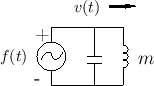
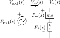
As discussed in Chapter 7 (§7.2), the equivalent
circuit for a force-driven mass is shown in Fig.F.10. The
mass ![]() is represented by an inductor
is represented by an inductor ![]() . The driving
force
. The driving
force ![]() is supplied via a voltage source, and the mass
velocity
is supplied via a voltage source, and the mass
velocity ![]() is the loop current.
is the loop current.
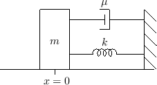
As also discussed in Chapter 7 (§7.2), if two physical elements are connected in such a way that they share a common velocity, then they are said to be formally connected in series. The ``series'' nature of the connection becomes more clear when the equivalent circuit is considered.
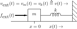
For example, Fig.1.9 shows a mass connected to one
end of a spring, with the other end of the spring attached to a rigid
wall. The driving force
![]() is applied to the mass
is applied to the mass ![]() on the left so that a positive force results in a positive mass
displacement
on the left so that a positive force results in a positive mass
displacement ![]() and positive spring displacement (compression)
and positive spring displacement (compression)
![]() . Since the mass and spring displacements are physically the
same, we can define
. Since the mass and spring displacements are physically the
same, we can define
![]() . Their velocities are
similarly equal so that
. Their velocities are
similarly equal so that
![]() . The equivalent circuit
has their electrical analogs connected in series, as shown in
Fig.1.10. The common mass and spring velocity
. The equivalent circuit
has their electrical analogs connected in series, as shown in
Fig.1.10. The common mass and spring velocity ![]() appear as a single current running through the inductor (mass) and
capacitor (spring).
appear as a single current running through the inductor (mass) and
capacitor (spring).
 |
By Kirchoff's loop law for circuit analysis, the sum of all voltages
around a loop equals zero.2.13 Thus, following
the direction for current ![]() in Fig.1.10, we have
in Fig.1.10, we have
![]() (where the minus sign for
(where the minus sign for
![]() occurs because the current enters its minus sign),
or
occurs because the current enters its minus sign),
or
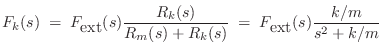
Impedance Networks
The concept of impedance is central in classical electrical
engineering. The simplest case is Ohm's Law for a resistor
![]() :
:
Thanks to the Laplace transform [449]2.15(or Fourier transform [451]),
the concept of impedance easily extends to masses and springs as well.
We need only allow impedances to be frequency-dependent. For
example, the Laplace transform of Newton's ![]() yields, using the
differentiation theorem for Laplace transforms [449],
yields, using the
differentiation theorem for Laplace transforms [449],
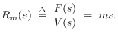
![\begin{eqnarray*}
R_k(s) &=& \frac{k}{s}\\ [5pt]
R_k(j\omega) &=& \frac{k}{j\omega}.
\end{eqnarray*}](http://www.dsprelated.com/josimages_new/pasp/img362.png)
The important benefit of this frequency-domain formulation of impedance is that it allows every interconnection of masses, springs, and dashpots (every RLC equivalent circuit) to be treated as a simple resistor network, parametrized by frequency.
 |
As an example, Fig.1.11 gives the impedance diagram corresponding to the equivalent circuit in Fig.1.10. Viewing the circuit as a (frequency-dependent) resistor network, it is easy to write down, say, the Laplace transform of the force across the spring using the voltage divider formula:
Wave Digital Filters
The idea of wave digital filters is to digitize RLC circuits (and certain more general systems) as follows:
- Determine the ODEs describing the system (PDEs also workable).
- Express all physical quantities (such as force and velocity) in
terms of traveling-wave components. The traveling wave
components are called wave variables. For example, the force
 on a mass is decomposed as
 , where
 is regarded as a traveling wave propagating toward
the mass, while
is regarded as a traveling wave propagating toward
the mass, while
 is seen as the traveling component
propagating away from the mass. A ``traveling wave'' view of
force mediation (at the speed of light) is actually much closer to
underlying physical reality than any instantaneous model.
is seen as the traveling component
propagating away from the mass. A ``traveling wave'' view of
force mediation (at the speed of light) is actually much closer to
underlying physical reality than any instantaneous model.
- Next, digitize the resulting traveling-wave system using the
bilinear transform (§7.3.2,[449, p. 386]).
The bilinear transform is equivalent in the time domain to the
trapezoidal rule for numerical integration (§7.3.2).
- Connect
 elementary units together by means of -port
scattering junctions. There are two basic types of scattering
junction, one for parallel, and one for series connection.
The theory of scattering junctions is introduced in the digital
waveguide context (§C.8).
elementary units together by means of -port
scattering junctions. There are two basic types of scattering
junction, one for parallel, and one for series connection.
The theory of scattering junctions is introduced in the digital
waveguide context (§C.8).
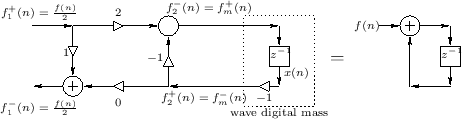
We will not make much use of WDFs in this book, preferring instead more prosaic finite-difference models for simplicity. However, we will utilize closely related concepts in the digital waveguide modeling context (Chapter 6).
Digital Waveguide Modeling Elements
As mentioned above, digital waveguide models are built out of digital delay-lines and filters (and nonlinear elements), and they can be understood as propagating and filtering sampled traveling-wave solutions to the wave equation (PDE), such as for air, strings, rods, and the like [433,437]. It is noteworthy that strings, woodwinds, and brasses comprise three of the four principal sections of a classical orchestra (all but percussion). The digital waveguide modeling approach has also been extended to propagation in 2D, 3D, and beyond [518,396,522,400]. They are not finite-difference models, but paradoxically they are equivalent under certain conditions (Appendix E). A summary of historical aspects appears in §A.9.
As mentioned at Eq.![]() (1.1), the ideal wave equation comes directly
from Newton's laws of motion (
(1.1), the ideal wave equation comes directly
from Newton's laws of motion (![]() ). For example, in the case of
vibrating strings, the wave equation is derived from first principles
(in Chapter 6, and more completely in Appendix C) to
be
). For example, in the case of
vibrating strings, the wave equation is derived from first principles
(in Chapter 6, and more completely in Appendix C) to
be
![\begin{eqnarray*}
Ky''&=& \epsilon {\ddot y}\\ [5pt]
\mbox{(Restoring Force Density} &=& \mbox{Mass Density times
Acceleration)}, \end{eqnarray*}](http://www.dsprelated.com/josimages_new/pasp/img369.png)
where
Defining
![]() , we obtain the usual form of the PDE known as
the ideal 1D wave equation.
, we obtain the usual form of the PDE known as
the ideal 1D wave equation.
where
![\begin{eqnarray*}
{\ddot y}& \isdef & \frac{\partial^2}{\partial t^2} y(t,x)\\ [5pt]
y''& \isdef & \frac{\partial^2}{\partial x^2} y(t,x).
\end{eqnarray*}](http://www.dsprelated.com/josimages_new/pasp/img375.png)
As has been known since d'Alembert [100], the 1D wave
equation is obeyed by arbitrary traveling waves at speed ![]() :
:
In digital waveguide modeling, the traveling-waves are sampled:
![\begin{eqnarray*}
y(nT,mX)
&=& y_r(nT-mX/c) + y_l(nT+mX/c)\qquad \mbox{(set $X=...
...y_r(nT-mT) + y_l(nT+mT)\\ [5pt]
&\isdef &y^{+}(n-m) + y^{-}(n+m)
\end{eqnarray*}](http://www.dsprelated.com/josimages_new/pasp/img379.png)
where ![]() denotes the time sampling interval in seconds,
denotes the time sampling interval in seconds, ![]() denotes the spatial sampling interval in meters, and
denotes the spatial sampling interval in meters, and ![]() and
and ![]() are defined for notational convenience.
are defined for notational convenience.
An ideal string (or air column) can thus be simulated using a
bidirectional delay line, as shown in
Fig.1.13 for the case of an ![]() -sample
section of ideal string or air column. The ``
-sample
section of ideal string or air column. The ``![]() '' label denotes its
wave impedance (§6.1.5) which is needed when connecting
digital waveguides to each other and to other kinds of computational
physical models (such as finite difference schemes). While
propagation speed on an ideal string is
'' label denotes its
wave impedance (§6.1.5) which is needed when connecting
digital waveguides to each other and to other kinds of computational
physical models (such as finite difference schemes). While
propagation speed on an ideal string is
![]() , we will
derive (§C.7.3) that the wave impedance is
, we will
derive (§C.7.3) that the wave impedance is
![]() .
.
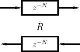 |
Figure 1.14 (from Chapter 6,
§6.3), illustrates a simple digital waveguide model for
rigidly terminated vibrating strings (more specifically, one
polarization-plane of transverse vibration). The traveling-wave
components are taken to be displacement samples, but the
diagram for velocity-wave and acceleration-wave simulation are
identical (inverting reflection at each rigid termination). The
output signal ![]() is formed by summing traveling-wave
components at the desired ``virtual pickup'' location (position
is formed by summing traveling-wave
components at the desired ``virtual pickup'' location (position
![]() in this example). To drive the string at a particular point,
one simply takes the transpose [449] of the output sum,
i.e., the input excitation is summed equally into the left- and
right-going delay-lines at the same
in this example). To drive the string at a particular point,
one simply takes the transpose [449] of the output sum,
i.e., the input excitation is summed equally into the left- and
right-going delay-lines at the same ![]() position (details will be
discussed near Fig.6.14).
position (details will be
discussed near Fig.6.14).
![\includegraphics[width=\twidth]{eps/fterminatedstringCopy}](http://www.dsprelated.com/josimages_new/pasp/img386.png) |
In Chapter 9 (example applications), we will discuss digital waveguide models for single-reed instruments such as the clarinet (Fig.1.15), and bowed-string instruments (Fig.1.16) such as the violin.
![\includegraphics[width=\twidth]{eps/fSingleReedWGMCopy}](http://www.dsprelated.com/josimages_new/pasp/img387.png) |
![\includegraphics[width=\twidth]{eps/fBowedStringsWGMCopy}](http://www.dsprelated.com/josimages_new/pasp/img388.png)
General Modeling Procedure
While each situation tends to have special opportunities, the following procedure generally works well:
- Formulate a state-space model.
- If it is nonlinear, use numerical time-integration:
- Explicit (causal finite difference scheme)
- Implicit (iteratively solved each time step)
- Semi-Implicit (truncated iterations of Implicit)
- In the linear case, diagonalize the state-space model to obtain
the modal representation.
- Implement isolated modes as second-order filters (``biquads'').
- Implement quasi-harmonic mode series as digital waveguides.
Next Section:
Our Plan
Previous Section:
Signal Models


