


Variable Filter Parametrizations
In practical applications of Lagrange Fractional-Delay Filtering
(LFDF), it is typically necessary to compute the FIR interpolation
coefficients
![]() as a function of the desired delay
as a function of the desired delay
![]() , which is usually time varying. Thus, LFDF is a special case
of FIR variable filtering in which the FIR coefficients must be
time-varying functions of a single delay parameter
, which is usually time varying. Thus, LFDF is a special case
of FIR variable filtering in which the FIR coefficients must be
time-varying functions of a single delay parameter ![]() .
.
Table Look-Up
A general approach to variable filtering is to tabulate the filter
coefficients as a function of the desired variables. In the case of
fractional delay filters, the impulse response
![]() is
tabulated as a function of delay
is
tabulated as a function of delay
![]() ,
,
![]() ,
,
![]() , where
, where ![]() is the
interpolation-filter order. For each
is the
interpolation-filter order. For each ![]() ,
, ![]() may be sampled
sufficiently densely so that linear interpolation will give a
sufficiently accurate ``interpolated table look-up'' of
may be sampled
sufficiently densely so that linear interpolation will give a
sufficiently accurate ``interpolated table look-up'' of
![]() for each
for each ![]() and (continuous)
and (continuous) ![]() . This method is commonly used
in closely related problem of sampling-rate conversion
[462].
. This method is commonly used
in closely related problem of sampling-rate conversion
[462].
Polynomials in the Delay
A more parametric approach is to formulate each filter coefficient
![]() as a polynomial in the desired delay
as a polynomial in the desired delay ![]() :
:
Taking the z transform of this expression leads to the interesting and useful Farrow structure for variable FIR filters [134].
Farrow Structure
Taking the z transform of Eq.![]() (4.9) yields
(4.9) yields
![$\displaystyle \sum_{n=0}^N \left[\sum_{m=0}^M c_n(m)\Delta^m\right]z^{-n}$](http://www.dsprelated.com/josimages_new/pasp/img1079.png)
![$\displaystyle \sum_{m=0}^M \left[\sum_{n=0}^N c_n(m) z^{-n}\right]\Delta^m$](http://www.dsprelated.com/josimages_new/pasp/img1080.png)
Since
Such a parametrization of a variable filter as a polynomial in
fixed filters ![]() is called a Farrow structure
[134,502]. When the polynomial Eq.
is called a Farrow structure
[134,502]. When the polynomial Eq.![]() (4.10) is
evaluated using Horner's rule,5.5 the efficient structure of
Fig.4.19 is obtained. Derivations of Farrow-structure
coefficients for Lagrange fractional-delay filtering are introduced in
[502, §3.3.7].
(4.10) is
evaluated using Horner's rule,5.5 the efficient structure of
Fig.4.19 is obtained. Derivations of Farrow-structure
coefficients for Lagrange fractional-delay filtering are introduced in
[502, §3.3.7].
![\includegraphics[width=\twidth]{eps/farrow}](http://www.dsprelated.com/josimages_new/pasp/img1087.png) |
As we will see in the next section, Lagrange interpolation can be
implemented exactly by the Farrow structure when ![]() . For
. For ![]() ,
approximations that do not satisfy the exact interpolation property
can be computed [148].
,
approximations that do not satisfy the exact interpolation property
can be computed [148].
Farrow Structure Coefficients
Beginning with a restatement of Eq.![]() (4.9),
(4.9),

![$\displaystyle h_\Delta(n) \eqsp
\underbrace{%
\left[\begin{array}{ccccc} 1 & \...
...y}{c} C_n(0) \\ [2pt] C_n(1) \\ [2pt] \vdots \\ [2pt] C_n(M)\end{array}\right]
$](http://www.dsprelated.com/josimages_new/pasp/img1090.png)
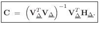
![$\displaystyle \underbrace{\left[\begin{array}{cccc}h_\Delta(0)\!&\!h_\Delta(1)\...
...\vdots \\
C_0(M) & C_1(M) & \cdots & C_N(M)
\end{array}\right]}_{\mathbf{C}}
$](http://www.dsprelated.com/josimages_new/pasp/img1091.png)
where
![$\displaystyle \mathbf{H}_{\underline{\Delta}}\isdefs \left[\begin{array}{c} \un...
...elta_0}^T \\ [2pt] \vdots \\ [2pt] \underline{h}_{\Delta_L}^T\end{array}\right]$](http://www.dsprelated.com/josimages_new/pasp/img1095.png) and
and![$\displaystyle \qquad
\mathbf{V}_{\underline{\Delta}}\isdefs \left[\begin{array}...
...ta_0}^T \\ [2pt] \vdots \\ [2pt] \underline{V}_{\Delta_L}^T\end{array}\right].
$](http://www.dsprelated.com/josimages_new/pasp/img1096.png)
Differentiator Filter Bank
Since, in the time domain, a Taylor series expansion of
![]() about time
about time ![]() gives
gives
![\begin{eqnarray*}
x(n-\Delta)
&=& x(n) -\Delta\, x^\prime(n)
+ \frac{\Delta^2...
...D^2(z) + \cdots
+ \frac{(-\Delta)^k}{k!}D^k(z) + \cdots \right]
\end{eqnarray*}](http://www.dsprelated.com/josimages_new/pasp/img1101.png)
where ![]() denotes the transfer function of the ideal differentiator,
we see that the
denotes the transfer function of the ideal differentiator,
we see that the ![]() th filter in Eq.
th filter in Eq.![]() (4.10) should approach
(4.10) should approach
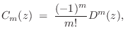
in the limit, as the number of terms
Farrow structures such as Fig.4.19 may be used to implement any
one-parameter filter variation in terms of several constant
filters. The same basic idea of polynomial expansion has been applied
also to time-varying filters (
![]() ).
).
Next Section:
Recent Developments in Lagrange Interpolation
Previous Section:
Proof of Maximum Flatness at DC


