


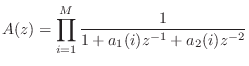
Virtual Musical Instruments
This chapter discusses aspects of synthesis models for specific musical instruments such as guitars, pianos, woodwinds, bowed strings, and brasses. Initially we look at model components for electric guitars, followed by some special considerations for acoustic guitars. Next we focus on basic models for string excitation, first by a mass (a simplified piano hammer), then by a damped spring (plectrum model). Piano modeling is then considered, using commuted synthesis for the acoustic resonators and a parametric signal-model for the force-pulse of the hammer. Finally, elementary synthesis of single-reed woodwinds, such as the clarinet, and bowed-string instruments, such as the violin, are summarized, and some pointers are given regarding other wind and percussion instruments.
Electric Guitars
For electric guitars, which are mainly about the vibrating string and subsequent effects processing, we pick up where §6.7 left off, and work our way up to practical complexity step by step. We begin with practical enhancements for the waveguide string model that are useful for all kinds of guitar models.
Length Three FIR Loop Filter
The simplest nondegenerate example of the loop filters of §6.8
is the three-tap FIR case (
![]() ). The symmetry constraint
leaves two degrees of freedom in the frequency response:10.1
). The symmetry constraint
leaves two degrees of freedom in the frequency response:10.1
Length  FIR Loop Filter Controlled by ``Brightness'' and ``Sustain''
Another convenient parametrization of the second-order symmetric FIR
case is when the dc normalization is relaxed so that two degrees of
freedom are retained. It is then convenient to control them
as brightness ![]() and sustain
and sustain ![]() according to the
formulas
according to the
formulas
where
One-Zero Loop Filter
If we relax the constraint that
![]() be odd, then the simplest case
becomes the one-zero digital filter:
be odd, then the simplest case
becomes the one-zero digital filter:
See [454] for related discussion from a software implementation perspective.
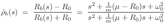
The Karplus-Strong Algorithm
The simulation diagram for the ideal string with the simplest frequency-dependent loss filter is shown in Fig. 9.1. Readers of the computer music literature will recognize this as the structure of the Karplus-Strong algorithm [236,207,489].
![\includegraphics[width=\twidth]{eps/fkarplusstrong}](http://www.dsprelated.com/josimages_new/pasp/img1962.png) |
The Karplus-Strong algorithm, per se, is obtained when the
delay-line initial conditions used to ``pluck'' the string consist of
random numbers, or ``white noise.'' We know the initial shape
of the string is obtained by adding the upper and lower delay
lines of Fig. 6.11, i.e.,
![]() . It is shown in §C.7.4 that the initial
velocity distribution along the string is determined by the
difference between the upper and lower delay lines. Thus, in
the Karplus-Strong algorithm, the string is ``plucked'' by a
random initial displacement and initial velocity distribution.
This is a very energetic excitation, and usually in practice the white
noise is lowpass filtered; the lowpass cut-off frequency gives an
effective dynamic level control since natural stringed
instruments are typically brighter at louder dynamic levels
[428,207].
. It is shown in §C.7.4 that the initial
velocity distribution along the string is determined by the
difference between the upper and lower delay lines. Thus, in
the Karplus-Strong algorithm, the string is ``plucked'' by a
random initial displacement and initial velocity distribution.
This is a very energetic excitation, and usually in practice the white
noise is lowpass filtered; the lowpass cut-off frequency gives an
effective dynamic level control since natural stringed
instruments are typically brighter at louder dynamic levels
[428,207].
Karplus-Strong sound examples are available on the Web.
An implementation of the Karplus-Strong algorithm in the Faust programming language is described (and provided) in [454].
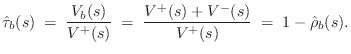
The Extended Karplus-Strong Algorithm
Figure 9.2 shows a block diagram of the Extended Karplus-Strong (EKS) algorithm [207].
![\includegraphics[width=\twidth]{eps/eks}](http://www.dsprelated.com/josimages_new/pasp/img1964.png)
The EKS adds the following features to the KS algorithm:
where
Note that while
![]() can be used in the tuning allpass, it
is better to offset it to
can be used in the tuning allpass, it
is better to offset it to
![]() to avoid delays
close to zero in the tuning allpass. (A zero delay is obtained by a
pole-zero cancellation on the unit circle.) First-order allpass
interpolation of delay lines was discussed in §4.1.2.
to avoid delays
close to zero in the tuning allpass. (A zero delay is obtained by a
pole-zero cancellation on the unit circle.) First-order allpass
interpolation of delay lines was discussed in §4.1.2.
A history of the Karplus-Strong algorithm and its extensions is given
in §A.8. EKS sound
examples
are also available on the Web. Techniques for designing the
string-damping filter ![]() and/or the string-stiffness allpass
filter
and/or the string-stiffness allpass
filter ![]() are summarized below in §6.11.
are summarized below in §6.11.
An implementation of the Extended Karplus-Strong (EKS) algorithm in the Faust programming language is described (and provided) in [454].
Nonlinear Distortion
In §6.13, nonlinear elements were introduced in the context of general digital waveguide synthesis. In this section, we discuss specifically virtual electric guitar distortion, and mention other instances of audible nonlinearity in stringed musical instruments.
As discussed in Chapter 6, typical vibrating strings in musical acoustics are well approximated as linear, time-invariant systems, there are special cases in which nonlinear behavior is desired.
Tension Modulation
In every freely vibrating string, the fundamental frequency declines
over time as the amplitude of vibration decays. This is due to
tension modulation, which is often audible at the beginning of
plucked-string tones, especially for low-tension strings. It happens
because higher-amplitude vibrations stretch the string to a
longer average length, raising the average string tension
![]() faster wave propagation
faster wave propagation
![]() higher fundamental
frequency.
higher fundamental
frequency.
The are several methods in the literature for simulating tension modulation in a digital waveguide string model [494,233,508,512,513,495,283], as well as in membrane models [298]. The methods can be classified into two categories, local and global.
Local tension-modulation methods modulate the speed of sound locally as a function of amplitude. For example, opposite delay cells in a force-wave digital waveguide string can be summed to obtain the instantaneous vertical force across that string sample, and the length of the adjacent propagation delay can be modulated using a first-order allpass filter. In principle the string slope reduces as the local tension increases. (Recall from Chapter 6 or Appendix C that force waves are minus the string tension times slope.)
Global tension-modulation methods [495,494] essentially modulate the string delay-line length as a function of the total energy in the string.
String Length Modulation
A number of stringed musical instruments have a ``nonlinear sound'' that comes from modulating the physical termination of the string (as opposed to its acoustic length in the case of tension modulation).
The Finnish Kantele [231,513] has a different effective string-length in the vertical and horizontal vibration planes due to a loose knot attaching the string to a metal bar. There is also nonlinear feeding of the second harmonic due to a nonrigid tuning peg.
Perhaps a better known example is the Indian sitar, in which a curved ``jawari'' (functioning as a nonlinear bridge) serves to shorten the string gradually as it displaces toward the bridge.
The Indian tambura also employs a thread perpendicular to the strings a short distance from the bridge, which serves to shorten the string whenever string displacement toward the bridge exceeds a certain distance.
Finally, the slap bass playing technique for bass guitars involves hitting the string hard enough to cause it to beat against the neck during vibration [263,366].
In all of these cases, the string length is physically modulated in some manner each period, at least when the amplitude is sufficiently large.
Hard Clipping
A widespread class of distortion used in electric guitars, is clipping of the guitar waveform. it is easy to add this effect to any string-simulation algorithm by passing the output signal through a nonlinear clipping function. For example, a hard clipper has the characteristic (in normalized form)
![$\displaystyle f(x) = \left\{\begin{array}{ll} -1, & x\leq -1 \\ [5pt] x, & -1 \leq x \leq 1 \\ [5pt] 1, & x\geq 1 \\ \end{array} \right. \protect$](http://www.dsprelated.com/josimages_new/pasp/img1514.png)
where
Soft Clipping
A soft clipper is similar to a hard clipper, but with the corners smoothed. A common choice of soft-clipper is the cubic nonlinearity, e.g. [489],
![$\displaystyle f(x) = \left\{\begin{array}{ll} -\frac{2}{3}, & x\leq -1 \\ [5pt]...
... \leq x \leq 1 \\ [5pt] \frac{2}{3}, & x\geq 1. \\ \end{array} \right. \protect$](http://www.dsprelated.com/josimages_new/pasp/img1970.png)
This particular soft-clipping characteristic is diagrammed in Fig.9.3. An analysis of its spectral characteristics, with some discussion of aliasing it may cause, was given in in §6.13. An input gain may be used to set the desired degree of distortion.
![\includegraphics[width=3in]{eps/cnl}](http://www.dsprelated.com/josimages_new/pasp/img1971.png)
Enhancing Even Harmonics
A cubic nonlinearity, as well as any odd distortion law,10.2 generates only odd-numbered harmonics (like in a square wave). For best results, and in particular for tube distortion simulation [31,395], it has been argued that some amount of even-numbered harmonics should also be present. Breaking the odd symmetry in any way will add even-numbered harmonics to the output as well. One simple way to accomplish this is to add an offset to the input signal, obtaining
Another method for breaking the odd symmetry is to add some square-law nonlinearity to obtain
where
Software for Cubic Nonlinear Distortion
The function cubicnl in the Faust software distribution (file effect.lib) implements cubic nonlinearity distortion [454]. The Faust programming example cubic_distortion.dsp provides a real-time demo with adjustable parameters, including an offset for bringing in even harmonics. The free, open-source guitarix application (for Linux platforms) uses this type of distortion effect along with many other guitar effects.
In the Synthesis Tool Kit (STK) [91], the class Cubicnl.cpp implements a general cubic distortion law.
Amplifier Feedback
A more extreme effect used with distorted electric guitars is amplifier feedback. In this case, the amplified guitar waveforms couple back to the strings with some gain and delay, as depicted schematically in Fig.9.4 [489].
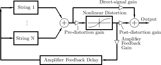
The Amplifier Feedback Delay in the figure can be adjusted to
emphasize certain partial overtones over others. If the loop gain,
controllable via the Amplifier Feedback Gain, is greater than 1 at any
frequency, a sustained ``feedback howl'' will be
produced. Note that in commercial devices, the Pre-distortion gain
and Post-distortion gain are frequency-dependent, i.e., they are
implemented as pre- and post-equalizers (typically only a few
bands, such as three). Another simple choice is an integrator
![]() for the pre-distortion gain, and a differentiator
for the pre-distortion gain, and a differentiator
![]() for the post-distortion gain.
for the post-distortion gain.
Faust software implementing electric-guitar amplifier feedback may be found in [454].
Cabinet Filtering
The distortion output signal is often further filtered by an amplifier cabinet filter, representing the enclosure, driver responses, etc. It is straightforward to measure the impulse response (or frequency response) of a speaker cabinet and fit it with a recursive digital filter design function such as invfreqz in matlab (§8.6.4). Individual speakers generally have one major resonance--the ``cone resonance''--which is determined by the mass, compliance, and damping of the driver subassembly. The enclosing cabinet introduces many more resonances in the audio range, generally tuned to even out the overall response as much as possible.
Faust software implementing an idealized speaker filter may be found in [454].
Duty-Cycle Modulation
For class A tube amplifier simulation, there should be level-dependent duty-cycle modulation as a function:10.3
- 50% at low amplitude levels (no duty-cycle modulation)
- 55-65% duty cycle at high levels
Vacuum Tube Modeling
The elementary nonlinearities discussed above are aimed at approximating the sound of amplifier distortion, such as often used by guitar players. Generally speaking, the distortion characteristics of vacuum-tube amplifiers are considered superior to those of solid-state amplifiers. A real-time numerically solved nonlinear differential algebraic model for class A single-ended guitar power amplification is presented in [84]. Real-time simulation of a tube guitar-amp (triode preamp, inverter, and push-pull amplifier) based on a precomputed approximate solution of the nonlinear differential equations is presented in [293]. Other references in this area include [338,228,339].
Acoustic Guitars
This section addresses some modeling considerations specific to acoustic guitars. Section 9.2.1 discusses special properties of acoustic guitar bridges, and §9.2.1 gives ways to simulate passive bridges, including a look at some laboratory measurements. For further reading in this area, see, e.g., [281,128].
Bridge Modeling
In §6.3 we analyzed the effect of rigid string terminations on traveling waves. We found that waves derived by time-derivatives of displacement (displacement, velocity, acceleration, and so on) reflect with a sign inversion, while waves defined in terms of the first spatial derivative of displacement (force, slope) reflect with no sign inversion. We now look at the more realistic case of yielding terminations for strings. This analysis can be considered a special case of the loaded string junction analyzed in §C.12.
Yielding string terminations (at the bridge) have a large effect on the sound produced by acoustic stringed instruments. Rigid terminations can be considered a reasonable model for the solid-body electric guitar in which maximum sustain is desired for played notes. Acoustic guitars, on the other hand, must transduce sound energy from the strings into the body of the instrument, and from there to the surrounding air. All audible sound energy comes from the string vibrational energy, thereby reducing the sustain (decay time) of each played note. Furthermore, because the bridge vibrates more easily in one direction than another, a kind of ``chorus effect'' is created from the detuning of the horizontal and vertical planes of string vibration (as discussed further in §6.12.1). A perfectly rigid bridge, in contrast, cannot transmit any sound into the body of the instrument, thereby requiring some other transducer, such as the magnetic pickups used in electric guitars, to extract sound for output.10.4
Passive String Terminations
When a traveling wave reflects from the bridge of a real stringed
instrument, the bridge moves, transmitting sound energy into the
instrument body. How far the bridge moves is determined by the
driving-point impedance of the bridge, denoted ![]() . The
driving point impedance is the ratio of Laplace transform of the force
on the bridge
. The
driving point impedance is the ratio of Laplace transform of the force
on the bridge ![]() to the velocity of motion that results
to the velocity of motion that results
![]() . That is,
. That is,
![]() .
.
For passive systems (i.e., for all unamplified acoustic musical
instruments), the driving-point impedance ![]() is positive
real (a property defined and discussed in §C.11.2). Being
positive real has strong implications on the nature of
is positive
real (a property defined and discussed in §C.11.2). Being
positive real has strong implications on the nature of ![]() . In
particular, the phase of
. In
particular, the phase of
![]() cannot exceed plus or minus
cannot exceed plus or minus
![]() degrees at any frequency, and in the lossless case, all poles and
zeros must interlace along the
degrees at any frequency, and in the lossless case, all poles and
zeros must interlace along the ![]() axis. Another
implication is that the reflectance of a passive bridge, as
seen by traveling waves on the string, is a so-called Schur
function (defined and discussed in §C.11); a Schur
reflectance is a stable filter having gain not exceeding 1 at any
frequency. In summary, a guitar bridge is passive if and only if its
driving-point impedance is positive real and (equivalently) its
reflectance is Schur. See §C.11 for a fuller discussion of
this point.
axis. Another
implication is that the reflectance of a passive bridge, as
seen by traveling waves on the string, is a so-called Schur
function (defined and discussed in §C.11); a Schur
reflectance is a stable filter having gain not exceeding 1 at any
frequency. In summary, a guitar bridge is passive if and only if its
driving-point impedance is positive real and (equivalently) its
reflectance is Schur. See §C.11 for a fuller discussion of
this point.
At ![]() , the force on the bridge is given by (§C.7.2)
, the force on the bridge is given by (§C.7.2)
A Terminating Resonator
Suppose a guitar bridge couples an ideal vibrating string to a single resonance, as depicted schematically in Fig.9.5. This is often an accurate model of an acoustic bridge impedance in a narrow frequency range, especially at low frequencies where the resonances are well separated. Then, as developed in Chapter 7, the driving-point impedance seen by the string at the bridge is
![\includegraphics[width=\twidth]{eps/f_yielding_term}](http://www.dsprelated.com/josimages_new/pasp/img1992.png) |
Bridge Reflectance
The bridge reflectance is needed as part of the loop filter in a digital waveguide model (Chapter 6).
As derived in §C.11.1, the force-wave reflectance of ![]() seen on the string is
seen on the string is
where
Bridge Transmittance
The bridge transmittance is the filter needed for the signal path from the vibrating string to the resonant acoustic body.
Since the bridge velocity equals the string endpoint velocity (a ``series'' connection), the velocity transmittance is simply
If the bridge is rigid, then its motion becomes a velocity input to the acoustic resonator. In principle, there are three such velocity inputs for each point along the bridge. However, it is typical in stringed instrument models to consider only the vertical transverse velocity on the string as significant, which results in one (vertical) driving velocity at the base of the bridge. In violin models (§9.6), the use of a ``sound post'' on one side of the bridge and ``bass bar'' on the other strongly suggests supporting a rocking motion along the bridge.
Digitizing Bridge Reflectance
Converting continuous-time transfer functions such as
![]() and
and
![]() to the digital domain is analogous to converting an analog
electrical filter to a corresponding digital filter--a problem which
has been well studied [343]. For this task, the
bilinear transform (§7.3.2) is a good choice. In
addition to preserving order and being free of aliasing, the bilinear
transform preserves the positive-real property of passive impedances
(§C.11.2).
to the digital domain is analogous to converting an analog
electrical filter to a corresponding digital filter--a problem which
has been well studied [343]. For this task, the
bilinear transform (§7.3.2) is a good choice. In
addition to preserving order and being free of aliasing, the bilinear
transform preserves the positive-real property of passive impedances
(§C.11.2).
Digitizing
![]() via the bilinear transform (§7.3.2)
transform gives
via the bilinear transform (§7.3.2)
transform gives
A Two-Resonance Guitar Bridge
Now let's consider a two-resonance guitar bridge, as shown in Fig. 9.6.
![\includegraphics[width=\twidth]{eps/lguitarsynth2simp2}](http://www.dsprelated.com/josimages_new/pasp/img2001.png) |
Like all mechanical systems that don't ``slide away'' in response to a
constant applied input force, the bridge must ``look like a spring''
at zero frequency. Similarly, it is typical for systems to ``look
like a mass'' at very high frequencies, because the driving-point
typically has mass (unless the driver is spring-coupled by what seems
to be massless spring). This implies the driving point admittance
should have a zero at dc and a pole at infinity. If we neglect
losses, as frequency increases up from zero, the first thing we
encounter in the admittance is a pole (a ``resonance'' frequency at
which energy is readily accepted by the bridge from the strings). As
we pass the admittance peak going up in frequency, the phase switches
around from being near ![]() (``spring like'') to being closer to
(``spring like'') to being closer to
![]() (``mass like''). (Recall the graphical method for
calculating the phase response of a linear system
[449].) Below the first resonance, we may say that the system
is stiffness controlled (admittance phase
(``mass like''). (Recall the graphical method for
calculating the phase response of a linear system
[449].) Below the first resonance, we may say that the system
is stiffness controlled (admittance phase
![]() ),
while above the first resonance, we say it is mass controlled
(admittance phase
),
while above the first resonance, we say it is mass controlled
(admittance phase
![]() ). This qualitative description is
typical of any lightly damped, linear, dynamic system. As we proceed
up the
). This qualitative description is
typical of any lightly damped, linear, dynamic system. As we proceed
up the ![]() axis, we'll next encounter a near-zero, or
``anti-resonance,'' above which the system again appears ``stiffness
controlled,'' or spring-like, and so on in alternation to infinity.
The strict alternation of poles and zeros near the
axis, we'll next encounter a near-zero, or
``anti-resonance,'' above which the system again appears ``stiffness
controlled,'' or spring-like, and so on in alternation to infinity.
The strict alternation of poles and zeros near the ![]() axis is
required by the positive real property of all passive
admittances (§C.11.2).
axis is
required by the positive real property of all passive
admittances (§C.11.2).
Measured Guitar-Bridge Admittance
![\includegraphics[width=\twidth]{eps/lguitardata}](http://www.dsprelated.com/josimages_new/pasp/img2004.png) |
A measured driving-point admittance [269]
for a real guitar bridge is shown in Fig. 9.7. Note
that at very low frequencies, the phase information does not appear to
be bounded by ![]() as it must be for the admittance to be
positive real (passive). This indicates a poor signal-to-noise ratio
in the measurements at very low frequencies. This can be verified by
computing and plotting the coherence function between the
bridge input and output signals using multiple physical
measurements.10.5
as it must be for the admittance to be
positive real (passive). This indicates a poor signal-to-noise ratio
in the measurements at very low frequencies. This can be verified by
computing and plotting the coherence function between the
bridge input and output signals using multiple physical
measurements.10.5
Figures 9.8 and 9.9 show overlays of the admittance magnitudes and phases, and also the input-output coherence, for three separate measurements. A coherence of 1 means that all the measurements are identical, while a coherence less than 1 indicates variation from measurement to measurement, implying a low signal-to-noise ratio. As can be seen in the figures, at frequencies for which the coherence is very close to 1, successive measurements are strongly in agreement, and the data are reliable. Where the coherence drops below 1, successive measurements disagree, and the measured admittance is not even positive real at very low frequencies.
![\includegraphics[width=\twidth]{eps/lguitarcoh}](http://www.dsprelated.com/josimages_new/pasp/img2006.png) |
![\includegraphics[width=\twidth]{eps/lguitarphs}](http://www.dsprelated.com/josimages_new/pasp/img2007.png) |
Building a Synthetic Guitar Bridge Admittance
To construct a synthetic guitar bridge model, we can first measure empirically the admittance of a real guitar bridge, or we can work from measurements published in the literature, as shown in Fig. 9.7. Each peak in the admittance curve corresponds to a resonance in the guitar body that is well coupled to the strings via the bridge. Whether or not the corresponding vibrational mode radiates efficiently depends on the geometry of the vibrational mode, and how well it couples to the surrounding air. Thus, a complete bridge model requires not only a synthetic bridge admittance which determines the reflectance ``seen'' on the string, but also a separate filter which models the transmittance from the bridge to the outside air; the transmittance filter normally contains the same poles as the reflectance filter, but the zeros are different. Moreover, keep in mind that each string sees a slightly different reflectance and transmittance because it is located at a slightly different point relative to the guitar top plate; this changes the coupling coefficients to the various resonating modes to some extent. (We normally ignore this for simplicity and use the same bridge filters for all the strings.)
Finally, also keep in mind that each string excites the bridge in three dimensions. The two most important are the horizontal and vertical planes of vibration, corresponding to the two planes of transverse vibration on the string. The vertical plane is normal to the guitar top plate, while the horizontal plane is parallel to the top plate. Longitudinal waves also excite the bridge, and they can be important as well, especially in the piano. Since longitudinal waves are much faster in strings than transverse waves, the corresponding overtones in the sound are normally inharmonically related to the main (nearly harmonic) overtones set up by the transverse string vibrations.
The frequency, complex amplitude, and width of each peak in the measured admittance of a guitar bridge can be used to determine the parameters of a second-order digital resonator in a parallel bank of such resonators being used to model the bridge impedance. This is a variation on modal synthesis [5,299]. However, for the bridge model to be passive when attached to a string, its transfer function must be positive real, as discused previously. Since strings are very nearly lossless, passivity of the bridge model is actually quite critical in practice. If the bridge model is even slightly active at some frequency, it can either make the whole guitar model unstable, or it might objectionably lengthen the decay time of certain string overtones.
We will describe two methods of constructing passive ``bridge filters'' from measured modal parameters. The first is guaranteed to be positive real but has some drawbacks. The second method gives better results, but it has to be checked for passivity and possibly modified to give a positive real admittance. Both methods illustrate more generally applicable signal processing methods.
Passive Reflectance Synthesis--Method 1
The first method is based on constructing a passive reflectance
![]() having the desired poles, and then converting to an
admittance via the fundamental relation
having the desired poles, and then converting to an
admittance via the fundamental relation
As we saw in §C.11.1, every passive impedance corresponds
to a passive reflectance which is a Schur function (stable and having gain
not exceeding ![]() around the unit circle). Since damping is light in a
guitar bridge impedance (otherwise the strings would not vibrate very long,
and sustain is a highly prized feature of real guitars), we can expect the
bridge reflectance to be close to an allpass transfer function
around the unit circle). Since damping is light in a
guitar bridge impedance (otherwise the strings would not vibrate very long,
and sustain is a highly prized feature of real guitars), we can expect the
bridge reflectance to be close to an allpass transfer function ![]() .
.
It is well known that every allpass transfer function can be expressed as
We will then construct a Schur function as
Recall that in every allpass filter with real coefficients, to every pole
at radius ![]() there corresponds a zero at radius
there corresponds a zero at radius ![]() .10.7
.10.7
Because the impedance is lightly damped, the poles and zeros of the
corresponding reflectance are close to the unit circle. This means that at
points along the unit circle between the poles, the poles and zeros tend to
cancel. It can be easily seen using the graphical method for computing the
phase of the frequency response that the pole-zero angles in the allpass
filter are very close to the resonance frequencies in the corresponding
passive impedance [429]. Furthermore, the distance of
the allpass poles to the unit circle controls the bandwidth of the
impedance peaks. Therefore, to a first approximation, we can treat the
allpass pole-angles as the same as those of the impedance pole angles, and
the pole radii in the allpass can be set to give the desired impedance peak
bandwidth. The zero-phase shaping filter ![]() gives the desired mode
height.
gives the desired mode
height.
From the measured peak frequencies ![]() and bandwidths
and bandwidths ![]() in the guitar
bridge admittance, we may approximate the pole locations
in the guitar
bridge admittance, we may approximate the pole locations
![]() as
as
where ![]() is the sampling interval as usual. Next we construct the
allpass denominator as the product of elementary second-order sections:
is the sampling interval as usual. Next we construct the
allpass denominator as the product of elementary second-order sections:
Now that we've constructed a Schur function, a passive admittance can be computed using (9.2.1). While it is guaranteed to be positive real, the modal frequencies, bandwidths, and amplitudes are only indirectly controlled and therefore approximated. (Of course, this would provide a good initial guess for an iterative procedure which computes an optimal approximation directly.)
A simple example of a synthetic bridge constructed using this method
with ![]() and
and ![]() is shown in Fig.9.10.
is shown in Fig.9.10.
![\includegraphics[width=\twidth]{eps/lguitarsynth}](http://www.dsprelated.com/josimages_new/pasp/img2028.png)
Passive Reflectance Synthesis--Method 2
The second method is based on constructing a partial fraction expansion of the admittance directly:
A simple example of a synthetic bridge constructed using this method with is shown in Fig.9.11.
![\includegraphics[width=\twidth]{eps/lguitarsynth2}](http://www.dsprelated.com/josimages_new/pasp/img2031.png)
Matlab for Passive Reflectance Synthesis Method 1
fs = 8192;  % Sampling rate in Hz (small for display convenience)
fc = 300;   % Upper frequency to look at
nfft = 8192;% FFT size (spectral grid density)

nspec = nfft/2+1;
nc = round(nfft*fc/fs);
f = ([0:nc-1]/nfft)*fs;

% Measured guitar body resonances
F = [4.64 96.52 189.33 219.95]; % frequencies
B = [ 10   10     10     10  ]; % bandwidths

nsec = length(F);

R = exp(-pi*B/fs);     % Pole radii
theta = 2*pi*F/fs;     % Pole angles
poles = R .* exp(j*theta);
A1 = -2*R.*cos(theta);  % 2nd-order section coeff
A2 = R.*R;              % 2nd-order section coeff
denoms = [ones(size(A1)); A1; A2]'
A = [1,zeros(1,2*nsec)];
for i=1:nsec,
    % polynomial multiplication = FIR filtering:
    A = filter(denoms(i,:),1,A);
end;
Now A contains the (stable) denominator of the desired bridge admittance. We want now to construct a numerator which gives a positive-real result. We'll do this by first creating a passive reflectance and then computing the corresponding PR admittance.
g = 0.9;         % Uniform loss factor

B = g*fliplr(A); % Flip(A)/A = desired allpass

Badm = A - B;
Aadm = A + B;
Badm = Badm/Aadm(1); % Renormalize
Aadm = Aadm/Aadm(1);

% Plots

fr = freqz(Badm,Aadm,nfft,'whole');

nc = round(nfft*fc/fs);
spec = fr(1:nc);
f = ([0:nc-1]/nfft)*fs;
dbmag = db(spec);
phase = angle(spec)*180/pi;

subplot(2,1,1);
plot(f,dbmag); grid;
title('Synthetic Guitar Bridge Admittance');
ylabel('Magnitude (dB)');
subplot(2,1,2);

plot(f,phase); grid;
ylabel('Phase (degrees)');
xlabel('Frequency (Hz)');
Matlab for Passive Reflectance Synthesis Method 2
... as in Method 1 for poles ...

% Construct a resonator as a sum of arbitrary modes
% with unit residues, adding a near-zero at dc.

B = zeros(1,2*nsec+1);
impulse = [1,zeros(1,2*nsec)];
for i=1:nsec,
    % filter() does polynomial division here:
    B = B + filter(A,denoms(i,:),impulse);
end;

% add a near-zero at dc
B = filter([1 -0.995],1,B);

... as in Method 1 for display ...
Matrix Bridge Impedance
A passive matrix bridge admittance (e.g., taking all six strings of the guitar together) can be conveniently synthesized as a vector of positive-real scalar admittances multiplied by a positive definite matrix [25]. In [25], a dual-polarization guitar-string model is connected to a matrix reflectance computed from the matrix driving-point impedance at the bridge.
Body Modeling
As introduced in §8.7, the commuted synthesis technique involves commuting the LTI filter representing acoustic resonator (guitar body) with the string, so that the string is excited by the pluck response of the body in place of the plectrum directly. The techniques described in §8.8 can be used to build practical computational synthesis models of acoustic guitar bodies and the like [229].
String Excitation
In §2.4 and §6.10 we looked at the basic architecture of a digital waveguide string excited by some external disturbance. We now consider the specific cases of string excitation by a hammer (mass) and plectrum (spring).
Ideal String Struck by a Mass
In §6.6, the ideal struck string was modeled as a simple initial velocity distribution along the string, corresponding to an instantaneous transfer of linear momentum from the striking hammer into the transverse motion of a string segment at time zero. (See Fig.6.10 for a diagram of the initial traveling velocity waves.) In that model, we neglected any effect of the striking hammer after time zero, as if it had bounced away at time 0 due to a so-called elastic collision. In this section, we consider the more realistic case of an inelastic collision, i.e., where the mass hits the string and remains in contact until something, such as a wave, or gravity, causes the mass and string to separate.
For simplicity, let the string length be infinity, and denote its wave
impedance by ![]() . Denote the colliding mass by
. Denote the colliding mass by ![]() and its speed
prior to collision by
and its speed
prior to collision by ![]() . It will turn out in this analysis that
we may approximate the size of the mass by zero (a so-called
point mass). Finally, we neglect the effects of gravity and
drag by the surrounding air. When the mass collides with the string,
our model must switch from two separate models (mass-in-flight and
ideal string), to that of two ideal strings joined by a mass
. It will turn out in this analysis that
we may approximate the size of the mass by zero (a so-called
point mass). Finally, we neglect the effects of gravity and
drag by the surrounding air. When the mass collides with the string,
our model must switch from two separate models (mass-in-flight and
ideal string), to that of two ideal strings joined by a mass ![]() at
at
![]() , as depicted in Fig.9.12. The ``force-velocity
port'' connections of the mass and two semi-infinite string endpoints
are formally in series because they all move together; that is,
the mass velocity equals the velocity of each of the two string
endpoints connected to the mass (see §7.2 for a fuller
discussion of impedances and their parallel/series connection).
, as depicted in Fig.9.12. The ``force-velocity
port'' connections of the mass and two semi-infinite string endpoints
are formally in series because they all move together; that is,
the mass velocity equals the velocity of each of the two string
endpoints connected to the mass (see §7.2 for a fuller
discussion of impedances and their parallel/series connection).
![\includegraphics[width=\twidth]{eps/massstringphy}](http://www.dsprelated.com/josimages_new/pasp/img2032.png)
The equivalent circuit for the mass-string assembly after time zero is
shown in Fig.9.13. Note that the string wave impedance ![]() appears twice, once for each string segment on the left and right.
Also note that there is a single common velocity
appears twice, once for each string segment on the left and right.
Also note that there is a single common velocity ![]() for the two
string endpoints and mass. LTI circuit elements in series can be
arranged in any order.
for the two
string endpoints and mass. LTI circuit elements in series can be
arranged in any order.
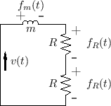 |
From the equivalent circuit, it is easy to solve for the velocity ![]() .
Formally, this is accomplished by applying Kirchoff's Loop Rule, which
states that the sum of voltages (``forces'') around any series loop is zero:
.
Formally, this is accomplished by applying Kirchoff's Loop Rule, which
states that the sum of voltages (``forces'') around any series loop is zero:
All of the signs are `
Taking the Laplace transform10.9of Eq.![]() (9.8) yields, by linearity,
(9.8) yields, by linearity,
where
For the mass, we have
![$\displaystyle f_m(t) = m\,a(t)\;=\; m\,\frac{d}{dt} v(t) \quad\longleftrightarrow\quad
F_m(s) = m\left[s\,V(s) - v_0\right],
$](http://www.dsprelated.com/josimages_new/pasp/img2043.png)
Substituting these relations into Eq.![]() (9.9) yields
(9.9) yields
We see that the initial momentum
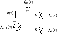 |
An advantage of the external-impulse formulation is that the system
has a zero initial state, so that an impedance description
(§7.1) is complete. In other words, the system can be
fully described as a series combination of the three impedances ![]() ,
,
![]() (on the left), and
(on the left), and ![]() (on the right), driven by an external
force-source
(on the right), driven by an external
force-source
![]() .
.
Solving Eq.![]() (9.10) for
(9.10) for ![]() yields
yields
The displacement of the string at ![]() is given by the integral of
the velocity:
is given by the integral of
the velocity:
![$\displaystyle y(t,0) = \int_0^t v(\tau)\,d\tau = v_0\,\frac{m}{2R}\,\left[1-e^{-{\frac{2R}{m}t}}\right]
$](http://www.dsprelated.com/josimages_new/pasp/img2056.png)
The momentum of the mass before time zero is ![]() , and after time
zero it is
, and after time
zero it is
The force applied to the two string endpoints by the mass is given by
![]() . From Newton's Law,
. From Newton's Law,
![]() , we have that
momentum
, we have that
momentum ![]() , delivered by the mass to the string,
can be calculated as the time integral of applied force:
, delivered by the mass to the string,
can be calculated as the time integral of applied force:
In a real piano, the hammer, which strikes in an upward (grand) or sideways (upright) direction, falls away from the string a short time after collision, but it may remain in contact with the string for a substantial fraction of a period (see §9.4 on piano modeling).
Mass Termination Model
The previous discussion solved for the motion of an ideal mass striking an ideal string of infinite length. We now investigate the same model from the string's point of view. As before, we will be interested in a digital waveguide (sampled traveling-wave) model of the string, for efficiency's sake (Chapter 6), and we therefore will need to know what the mass ``looks like'' at the end of each string segment. For this we will find that the impedance description (§7.1) is especially convenient.
![\includegraphics[width=\twidth]{eps/massstringphynum}](http://www.dsprelated.com/josimages_new/pasp/img2065.png) |
Let's number the string segments to the left and right of the mass by
1 and 2, respectively, as shown in Fig.9.15. Then
Eq.![]() (9.8) above may be written
(9.8) above may be written
where
To derive the traveling-wave relations in a digital waveguide model,
we want to use the force-wave variables
![]() and
and
![]() that we defined for vibrating strings in
§6.1.5; i.e., we defined
that we defined for vibrating strings in
§6.1.5; i.e., we defined
![]() , where
, where ![]() is the string tension and
is the string tension and ![]() is the string
slope,
is the string
slope, ![]() .
.
![\includegraphics[width=0.5\twidth]{eps/stringslope}](http://www.dsprelated.com/josimages_new/pasp/img2073.png) |
As shown in Fig.9.16, a negative string slope pulls ``up''
to the right. Therefore, at the mass point we have
![]() , where
, where ![]() denotes the position of the
mass along the string. On the other hand, the figure also shows that
a negative string slope pulls ``down'' to the left, so that
denotes the position of the
mass along the string. On the other hand, the figure also shows that
a negative string slope pulls ``down'' to the left, so that
![]() . In summary, relating the forces we
have defined for the mass-string junction to the force-wave variables
in the string, we have
. In summary, relating the forces we
have defined for the mass-string junction to the force-wave variables
in the string, we have
where ![]() denotes the position of the mass along the string.
denotes the position of the mass along the string.
Thus, we can rewrite Eq.![]() (9.11) in terms of string wave variables as
(9.11) in terms of string wave variables as
or, substituting the definitions of these forces,
The inertial force of the mass is
The force relations can be checked individually. For string 1,
Now that we have expressed the string forces in terms of string
force-wave variables, we can derive digital waveguide models by
performing the traveling-wave decompositions
![]() and
and
![]() and using the Ohm's law relations
and using the Ohm's law relations
![]() and
and
![]() for
for ![]() (introduced above near
Eq.
(introduced above near
Eq.![]() (6.6)).
(6.6)).
Mass Reflectance from Either String
Let's first consider how the mass looks from the viewpoint of string
1, assuming string 2 is at rest. In this situation (no incoming wave
from string 2), string 2 will appear to string 1 as a simple resistor
(or dashpot) of ![]() Ohms in series with the mass impedance
Ohms in series with the mass impedance ![]() .
(This observation will be used as the basis of a rapid solution method
in §9.3.1 below.)
.
(This observation will be used as the basis of a rapid solution method
in §9.3.1 below.)
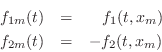
When a wave from string 1 hits the mass, it will cause the mass to move. This motion carries both string endpoints along with it. Therefore, both the reflected and transmitted waves include this mass motion. We can say that we see a ``dispersive transmitted wave'' on string 2, and a dispersive reflection back onto string 1. Our object in this section is to calculate the transmission and reflection filters corresponding to these transmitted and reflected waves.
By physical symmetry the velocity reflection and transmission
will be the same from string 1 as it is from string 2. We can say the
same about force waves, but we will be more careful because the sign
of the transverse force flips when the direction of travel is
reversed.10.12Thus, we expect a scattering junction of the form shown in
Fig.9.17 (recall the discussion of physically
interacting waveguide inputs in §2.4.3). This much invokes
the superposition principle (for simultaneous reflection and transmission),
and imposes the expected symmetry: equal reflection filters
![]() and
equal transmission filters
and
equal transmission filters
![]() (for either force or velocity waves).
(for either force or velocity waves).
![\includegraphics[width=\twidth]{eps/massstringdwmform1}](http://www.dsprelated.com/josimages_new/pasp/img2087.png) |
Let's begin with Eq.![]() (9.12) above, restated as follows:
(9.12) above, restated as follows:
The traveling-wave decompositions can be written out as
where a ``+'' superscript means ``right-going'' and a ``-'' superscript means ``left-going'' on either string.10.13
Let's define the mass position ![]() to be zero, so that Eq.
to be zero, so that Eq.![]() (9.14)
with the substitutions Eq.
(9.14)
with the substitutions Eq.![]() (9.15) becomes
(9.15) becomes
In the Laplace domain, dropping the common ``(s)'' arguments,
![\begin{eqnarray*}
F_m + F^{+}_1 + F^{-}_1 - F^{+}_2 -F^{-}_2 &=& 0\\ [10pt]
\Lon...
...row\quad
-msV + RV^{+}_1 - RV^{-}_1 - RV^{+}_2 + RV^{-}_2 &=& 0.
\end{eqnarray*}](http://www.dsprelated.com/josimages_new/pasp/img2101.png)
To compute the reflection coefficient of the mass seen on string 1, we
may set ![]() , which means
, which means
![]() , so that we have
, so that we have
From this, the reflected velocity is immediate:
It is always good to check that our answers make physical sense in
limiting cases. For this problem, easy cases to check are ![]() and
and
![]() . When the mass is
. When the mass is ![]() , the reflectance goes to zero (no
reflected wave at all). When the mass goes to infinity, the
reflectance approaches
, the reflectance goes to zero (no
reflected wave at all). When the mass goes to infinity, the
reflectance approaches
![]() , corresponding to a rigid
termination, which also makes sense.
, corresponding to a rigid
termination, which also makes sense.
The results of this section can be more quickly obtained as a special
case of the main result of §C.12, by choosing ![]() waveguides meeting at a load
impedance
waveguides meeting at a load
impedance ![]() . The next section gives another
fast-calculation method based on a standard formula.
. The next section gives another
fast-calculation method based on a standard formula.
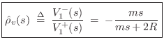
Simplified Impedance Analysis
The above results are quickly derived from the general reflection-coefficient for force waves (or voltage waves, pressure waves, etc.):
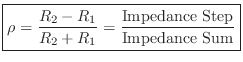
where
In the mass-string-collision problem, we can immediately write down the force reflectance of the mass as seen from either string:
Since, by the Ohm's-law relations,
Mass Transmittance from String to String
Referring to Fig.9.15, the velocity transmittance from string 1 to string 2 may be defined as


We can now refine the picture of our scattering junction Fig.9.17 to obtain the form shown in Fig.9.18.
![\includegraphics[width=0.8\twidth]{eps/massstringdwmformvel}](http://www.dsprelated.com/josimages_new/pasp/img2139.png) |
Force Wave Mass-String Model
The velocity transmittance is readily converted to a force transmittance using the Ohm's-law relations:
![\includegraphics[width=0.8\twidth]{eps/massstringdwmformforce}](http://www.dsprelated.com/josimages_new/pasp/img2142.png) |
Checking as before, we see that
![]() corresponds to
corresponds to
![]() , which means no force is transmitted through an
infinite mass, which is reasonable. As
, which means no force is transmitted through an
infinite mass, which is reasonable. As ![]() , the force
transmittance becomes 1 and the mass has no effect, as desired.
, the force
transmittance becomes 1 and the mass has no effect, as desired.
Summary of Mass-String Scattering Junction
In summary, we have characterized the mass on the string in terms of its reflectance and transmittance from either string. For force waves, we have outgoing waves given by

or
![$\displaystyle \left[\begin{array}{c} F^{+}_2 \\ [2pt] F^{-}_1 \end{array}\right...
...ay}\right] \left[\begin{array}{c} F^{+}_1 \\ [2pt] F^{-}_2 \end{array}\right]
$](http://www.dsprelated.com/josimages_new/pasp/img2144.png)
The one-filter form follows from the observation that
![]() appears in both computations, and therefore need only be implemented once:
appears in both computations, and therefore need only be implemented once:
![\begin{eqnarray*}
F^{+}&\isdef & \hat{\rho}_f\cdot(F^{+}_1+F^{-}_2)\\ [5pt]
F^{-}_1 &=& F^{-}_2 + F^{+}\\ [5pt]
F^{+}_2 &=& F^{+}_1 + F^{+}
\end{eqnarray*}](http://www.dsprelated.com/josimages_new/pasp/img2152.png)
This structure is diagrammed in Fig.9.20.
![\includegraphics[width=\twidth]{eps/massstringdwms}](http://www.dsprelated.com/josimages_new/pasp/img2153.png) |
Again, the above results follow immediately from the more general formulation of §C.12.
Digital Waveguide Mass-String Model
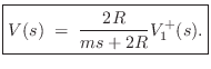
To obtain a force-wave digital waveguide model of the string-mass assembly after the mass has struck the string, it only remains to digitize the model of Fig.9.20. The delays are obviously to be implemented using digital delay lines. For the mass, we must digitize the force reflectance appearing in the one-filter model of Fig.9.20:
A common choice of digitization method is the bilinear transform (§7.3.2) because it preserves losslessness and does not alias. This will effectively yield a wave digital filter model for the mass in this context (see Appendix F for a tutorial on wave digital filters).
The bilinear transform is typically scaled as
![\begin{eqnarray*}
\hat{\rho}_d(z)
&=& \frac{1}{1+\frac{2R}{m}\frac{T}{2}\frac{1+z^{-1}}{1-z^{-1}}}\\ [5pt]
&=& g\frac{1-z^{-1}}{1-pz^{-1}}
\end{eqnarray*}](http://www.dsprelated.com/josimages_new/pasp/img2157.png)
where the gain coefficient ![]() and pole
and pole ![]() are given by
are given by
![\begin{eqnarray*}
g&\isdef &\frac{1}{1+\frac{RT}{m}}\;<\;1\\ [5pt]
p&\isdef &\frac{1-\frac{RT}{m}}{1+\frac{RT}{m}}\;<\;1.
\end{eqnarray*}](http://www.dsprelated.com/josimages_new/pasp/img2158.png)
Thus, the reflectance of the mass is a one-pole, one-zero filter. The
zero is exactly at dc, the real pole is close to dc, and the gain at
half the sampling rate is ![]() . We may recognize this as the classic
dc-blocking filter
[449]. Comparing with Eq.
. We may recognize this as the classic
dc-blocking filter
[449]. Comparing with Eq.![]() (9.18), we see that the behavior
at dc is correct, and that the behavior at infinite frequency
(
(9.18), we see that the behavior
at dc is correct, and that the behavior at infinite frequency
(
![]() ) is now the behavior at half the sampling rate
(
) is now the behavior at half the sampling rate
(
![]() ).
).
Physically, the mass reflectance is zero at dc because sufficiently slow waves can freely move a mass of any finite size. The reflectance is 1 at infinite frequency because there is no time for the mass to start moving before it is pushed in the opposite direction. In short, a mass behaves like a rigid termination at infinite frequency, and a free end (no termination) at zero frequency. The reflectance of a mass is therefore a ``dc blocker''.
The final digital waveguide model of the mass-string combination is shown in Fig.9.21.
![\includegraphics[width=\twidth]{eps/massstringdwmz}](http://www.dsprelated.com/josimages_new/pasp/img2161.png)
Additional examples of lumped-element modeling, including masses, springs, dashpots, and their various interconnections, are discussed the Wave Digital Filters (WDF) appendix (Appendix F). A nice feature WDFs is that they employ traveling-wave input/output signals which are ideal for interfacing to digital waveguides. The main drawback is that the WDFs operate over a warped frequency axis (due to the bilinear transform), while digital delay lines have a normal (unwarped) frequency axis. On the plus side, WDFs cannot alias, while digital waveguides do alias in the frequency domain for signals that are not bandlimited to less than half the sampling rate. At low frequencies (or given sufficient oversampling), the WDF frequency warping is minimal, and in such cases, WDF ``lumped element models'' may be connected directly to digital waveguides, which are ``sampled-wave distributed parameter'' models.
Even when the bilinear-transform frequency-warping is severe, it is often well tolerated when the frequency response has only one ``important frequency'', such as a second-order resonator, lowpass, or highpass response. In other words, the bilinear transform can be scaled to map any single analog frequency to any desired corresponding digital frequency (see §7.3.2 for details), and the frequency-warped responses above and below the exactly mapped frequency may ``sound as good as'' the unwarped responses for musical purposes. If not, higher order filters can be used to model lumped elements (Chapter 7).
Displacement-Wave Simulation
As discussed in [121], displacement waves
are often preferred over force or velocity waves for guitar-string
simulations, because such strings often hit obstacles such as frets or
the neck. To obtain displacement from velocity at a given ![]() ,
we may time-integrate
velocity as above to produce displacement at any spatial sample along the
string where a collision might be possible. However, all these
integrators can be eliminated by simply going to a displacement-wave
simulation, as has been done in nearly all papers to date on plucking
models for digital waveguide strings.
,
we may time-integrate
velocity as above to produce displacement at any spatial sample along the
string where a collision might be possible. However, all these
integrators can be eliminated by simply going to a displacement-wave
simulation, as has been done in nearly all papers to date on plucking
models for digital waveguide strings.
To convert our force-wave simulation to a displacement-wave
simulation, we may first convert force to velocity using the Ohm's law
relations
![]() and
and
![]() and then
conceptually integrate all signals with respect to time (in advance of
the simulation).
and then
conceptually integrate all signals with respect to time (in advance of
the simulation).
![]() is the same on both sides of the finger-junction, which means we
can convert from force to velocity by simply negating all left-going
signals. (Conceptually, all signals are converted from force to
velocity by the Ohm's law relations and then divided by
is the same on both sides of the finger-junction, which means we
can convert from force to velocity by simply negating all left-going
signals. (Conceptually, all signals are converted from force to
velocity by the Ohm's law relations and then divided by ![]() , but the
common scaling by
, but the
common scaling by ![]() can be omitted (or postponed) unless signal
values are desired in particular physical units.) An
all-velocity-wave simulation can be converted to displacement waves
even more easily by simply changing
can be omitted (or postponed) unless signal
values are desired in particular physical units.) An
all-velocity-wave simulation can be converted to displacement waves
even more easily by simply changing ![]() to
to ![]() everywhere, because
velocity and displacement waves scatter identically. In more general
situations, we can go to the Laplace domain and replace each
occurrence of
everywhere, because
velocity and displacement waves scatter identically. In more general
situations, we can go to the Laplace domain and replace each
occurrence of ![]() by
by ![]() , each
, each ![]() by
by ![]() ,
divide all signals by
,
divide all signals by ![]() , push any leftover
, push any leftover ![]() around for maximum
simplification, perhaps absorbing it into a nearby filter. In an
all-velocity-wave simulation, each signal gets multiplied by
around for maximum
simplification, perhaps absorbing it into a nearby filter. In an
all-velocity-wave simulation, each signal gets multiplied by ![]() in
this procedure, which means it cancels out of all definable transfer
functions. All filters in the diagram (just
in
this procedure, which means it cancels out of all definable transfer
functions. All filters in the diagram (just
![]() in this
example) can be left alone because their inputs and outputs are still
force-valued in principle. (We expressed each force wave in terms of
velocity and wave impedance without changing the signal flow diagram,
which remains a force-wave simulation until minus signs, scalings, and
in this
example) can be left alone because their inputs and outputs are still
force-valued in principle. (We expressed each force wave in terms of
velocity and wave impedance without changing the signal flow diagram,
which remains a force-wave simulation until minus signs, scalings, and
![]() operators are moved around and combined.) Of course, one can
absorb scalings and sign reversals into the filter(s) to change the
physical input/output units as desired. Since we routinely assume
zero initial conditions in an impedance description, the integration
constants obtained by time-integrating velocities to get displacements
are all defined to be zero. Additional considerations regarding the
choice of displacement waves over velocity (or force) waves are given
in §E.3.3. In particular, their initial conditions can be very
different, and traveling-wave components tend not to be as well
behaved for displacement waves.
operators are moved around and combined.) Of course, one can
absorb scalings and sign reversals into the filter(s) to change the
physical input/output units as desired. Since we routinely assume
zero initial conditions in an impedance description, the integration
constants obtained by time-integrating velocities to get displacements
are all defined to be zero. Additional considerations regarding the
choice of displacement waves over velocity (or force) waves are given
in §E.3.3. In particular, their initial conditions can be very
different, and traveling-wave components tend not to be as well
behaved for displacement waves.
Piano Hammer Modeling
The previous section treated an ideal point-mass striking an ideal string. This can be considered a simplified piano-hammer model. The model can be improved by adding a damped spring to the point-mass, as shown in Fig.9.22 (cf. Fig.9.12).
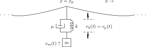 |
The impedance of this plucking system, as seen by the string, is the
parallel combination of the mass impedance ![]() and the damped spring
impedance
and the damped spring
impedance ![]() . (The damper
. (The damper ![]() and spring
and spring ![]() are formally
in series--see §7.2, for a refresher on series versus
parallel connection.) Denoting
the driving-point impedance of the hammer at the string contact-point
by
are formally
in series--see §7.2, for a refresher on series versus
parallel connection.) Denoting
the driving-point impedance of the hammer at the string contact-point
by ![]() , we have
, we have
Thus, the scattering filters in the digital waveguide model are second order (biquads), while for the string struck by a mass (§9.3.1) we had first-order scattering filters. This is expected because we added another energy-storage element (a spring).
The impedance formulation of Eq.![]() (9.19) assumes all elements are
linear and time-invariant (LTI), but in practice one can normally
modulate element values as a function of time and/or state-variables
and obtain realistic results for low-order elements. For this we must
maintain filter-coefficient formulas that are explicit functions of
physical state and/or time. For best results, state variables should
be chosen so that any nonlinearities remain memoryless in the
digitization
[361,348,554,555].
(9.19) assumes all elements are
linear and time-invariant (LTI), but in practice one can normally
modulate element values as a function of time and/or state-variables
and obtain realistic results for low-order elements. For this we must
maintain filter-coefficient formulas that are explicit functions of
physical state and/or time. For best results, state variables should
be chosen so that any nonlinearities remain memoryless in the
digitization
[361,348,554,555].
Nonlinear Spring Model
In the musical acoustics literature, the piano hammer is classically
modeled as a nonlinear spring
[493,63,178,76,60,486,164].10.14Specifically, the piano-hammer damping in Fig.9.22 is
typically approximated by ![]() , and the spring
, and the spring ![]() is
nonlinear and memoryless according to a simple power
law:
is
nonlinear and memoryless according to a simple power
law:
The upward force applied to the string by the hammer is therefore
| (10.20) |
This force is balanced at all times by the downward string force (string tension times slope difference), exactly as analyzed in §9.3.1 above.
Including Hysteresis
Since the compressed hammer-felt (wool) on real piano hammers shows significant hysteresis memory, an improved piano-hammer felt model is
![$\displaystyle f_h(t) \eqsp Q_0\left[x_k^p + \alpha \frac{d(x_k^p)}{dt}\right], \protect$](http://www.dsprelated.com/josimages_new/pasp/img2177.png)
where
Equation (9.21) is said to be a good approximation under normal playing conditions. A more complete hysteresis model is [487]
![$\displaystyle f_h(t) \eqsp f_0\left[x_k^p(t) - \frac{\epsilon}{\tau_0} \int_0^t x_k^p(\xi) \exp\left(\frac{\xi-t}{\tau_0}\right)d\xi\right]
$](http://www.dsprelated.com/josimages_new/pasp/img2179.png)
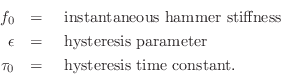
Relating to Eq.![]() (9.21) above, we have
(9.21) above, we have
![]() (N/mm
(N/mm![]() ).
).
Piano Hammer Mass
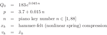
The piano-hammer mass may be approximated across the keyboard by [487]
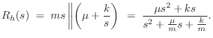
Pluck Modeling
The piano-hammer model of the previous section can also be configured
as a plectrum by making the mass and damping small or zero, and
by releasing the string when the contact force exceeds some threshold
![]() . That is, to a first approximation, a plectrum can be modeled
as a spring (linear or nonlinear) that disengages when either
it is far from the string or a maximum spring-force is exceeded. To
avoid discontinuities when the plectrum and string engage/disengage,
it is good to taper both the damping and spring-constant to zero at
the point of contact (as shown
below).
. That is, to a first approximation, a plectrum can be modeled
as a spring (linear or nonlinear) that disengages when either
it is far from the string or a maximum spring-force is exceeded. To
avoid discontinuities when the plectrum and string engage/disengage,
it is good to taper both the damping and spring-constant to zero at
the point of contact (as shown
below).
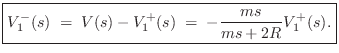
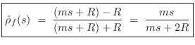
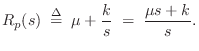
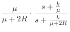
Starting with the piano-hammer impedance of Eq.![]() (9.19) and setting
the mass
(9.19) and setting
the mass ![]() to infinity (the plectrum holder is immovable), we define
the plectrum impedance as
to infinity (the plectrum holder is immovable), we define
the plectrum impedance as
The force-wave reflectance of impedance ![]() in Eq.
in Eq.![]() (9.22), as
seen from the string, may be computed exactly as in
§9.3.1:
(9.22), as
seen from the string, may be computed exactly as in
§9.3.1:
![$\displaystyle \frac{\mbox{Impedance Step}}{\mbox{Impedance Sum}}
\eqsp \frac{[R_p(s)+R]-R}{[R_p(s)+R]+R}
\eqsp \frac{R_p(s)}{R_p(s)+2R}$](http://www.dsprelated.com/josimages_new/pasp/img2187.png)
If the spring damping is much greater than twice the string wave impedance (
Again following §9.3.1, the transmittance for force waves is given by
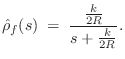
If the damping ![]() is set to zero, i.e., if the plectrum is to be modeled
as a simple linear spring, then the impedance becomes
is set to zero, i.e., if the plectrum is to be modeled
as a simple linear spring, then the impedance becomes
![]() ,
and the force-wave reflectance becomes
[128]
,
and the force-wave reflectance becomes
[128]
Digital Waveguide Plucked-String Model
When plucking a string, it is necessary to detect ``collisions''
between the plectrum and string. Also, more complete plucked-string
models will allow the string to ``buzz'' on the frets and ``slap''
against obstacles such as the fingerboard. For these reasons, it is
convenient to choose displacement waves for the waveguide
string model. The reflection and transmission filters for
displacement waves are the same as for velocity, namely,
![]() and
and
![]() .
.
As in the mass-string collision case, we obtain the one-filter
scattering-junction implementation shown in Fig.9.23. The filter
![]() may now be digitized using the bilinear transform as
previously (§9.3.1).
may now be digitized using the bilinear transform as
previously (§9.3.1).
Incorporating Control Motion
Let ![]() denote the vertical position of the mass
in Fig.9.22. (We still assume
denote the vertical position of the mass
in Fig.9.22. (We still assume ![]() .) We can think of
.) We can think of
![]() as the position of the control point on the
plectrum, e.g., the position of the ``pinch-point'' holding the
plectrum while plucking the string. In a harpsichord,
as the position of the control point on the
plectrum, e.g., the position of the ``pinch-point'' holding the
plectrum while plucking the string. In a harpsichord, ![]() can be
considered the jack position [347].
can be
considered the jack position [347].
Also denote by ![]() the rest length of the spring
the rest length of the spring ![]() in Fig.9.22, and let
in Fig.9.22, and let
![]() denote the
position of the ``end'' of the spring while not in contact with the
string. Then the plectrum makes contact with the string when
denote the
position of the ``end'' of the spring while not in contact with the
string. Then the plectrum makes contact with the string when
Let the subscripts ![]() and
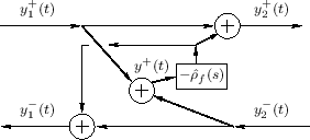
and ![]() each denote one side of the scattering
system, as indicated in Fig.9.23. Then, for example,
each denote one side of the scattering
system, as indicated in Fig.9.23. Then, for example,
![]() is the displacement of the string on the left (side
is the displacement of the string on the left (side
![]() ) of plucking point, and
) of plucking point, and ![]() is on the right side of
is on the right side of ![]() (but
still located at point
(but
still located at point ![]() ). By continuity of the string, we have
). By continuity of the string, we have
When the spring engages the string (![]() ) and begins to compress,
the upward force on the string at the contact point is given by
) and begins to compress,
the upward force on the string at the contact point is given by
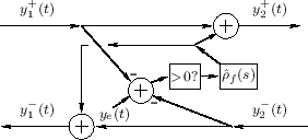
During contact, force equilibrium at the plucking point requires (cf. §9.3.1)
where
Substituting
![]() and taking the Laplace transform yields
and taking the Laplace transform yields
![$\displaystyle Y(s)
\eqsp Y_1^+(s) + Y_2^-(s) + \frac{1}{2R} \frac{F_k(s)}{s}
\eqsp Y_1^+(s) + Y_2^-(s) + \frac{k}{2Rs}\left[Y_e(s) - Y(s)\right].
$](http://www.dsprelated.com/josimages_new/pasp/img2224.png)
![\begin{eqnarray*}
Y(s) &=& \left[1-\hat{\rho}_f(s)\right]\cdot
\left[Y_1^+(s)+Y...
...)\cdot \left\{Y_e(s)
- \left[Y_1^+(s)+Y_2^-(s)\right]\right\},
\end{eqnarray*}](http://www.dsprelated.com/josimages_new/pasp/img2226.png)
where, as first noted at Eq.![]() (9.24) above,
(9.24) above,

![\begin{eqnarray*}
Y_d^+ &=& Y_e - \left(Y_1^+ + Y_2^-\right)\\ [5pt]
Y_1^- &=& Y...
...\hat{\rho}_f Y_d^+\\ [5pt]
Y_2^+ &=& Y_1^+ + \hat{\rho}_f Y_d^+.
\end{eqnarray*}](http://www.dsprelated.com/josimages_new/pasp/img2228.png)
This system is diagrammed in Fig.9.24. The manipulation of the
minus signs relative to Fig.9.23 makes it convenient for
restricting ![]() to positive values only (as shown in the
figure), corresponding to the plectrum engaging the string going up.
This uses the approximation
to positive values only (as shown in the
figure), corresponding to the plectrum engaging the string going up.
This uses the approximation
![]() ,
which is exact when
,
which is exact when
![]() , i.e., when the plectrum does not affect
the string displacement at the current time. It is therefore exact at
the time of collision and also applicable just after release.
Similarly,
, i.e., when the plectrum does not affect
the string displacement at the current time. It is therefore exact at
the time of collision and also applicable just after release.
Similarly,
![]() can be used to trigger a release of the
string from the plectrum.
can be used to trigger a release of the
string from the plectrum.
Successive Pluck Collision Detection
As discussed above, in a simple 1D plucking model, the plectrum comes
up and engages the string when
![]() , and above some
maximum force the plectrum releases the string. At this point, it is
``above'' the string. To pluck again in the same direction, the
collision-detection must be disabled until we again have
, and above some
maximum force the plectrum releases the string. At this point, it is
``above'' the string. To pluck again in the same direction, the
collision-detection must be disabled until we again have ![]() ,
requiring one bit of state to keep track of that.10.16 The harpsichord jack
plucks the string only in the ``up'' direction due to its asymmetric
behavior in the two directions [143]. If only
``up picks'' are supported, then engagement can be suppressed after a
release until
,
requiring one bit of state to keep track of that.10.16 The harpsichord jack
plucks the string only in the ``up'' direction due to its asymmetric
behavior in the two directions [143]. If only
``up picks'' are supported, then engagement can be suppressed after a
release until ![]() comes back down below the envelope of string
vibration (e.g.,
comes back down below the envelope of string
vibration (e.g.,
![]() ). Note that
intermittent disengagements as a plucking cycle begins are normal;
there is often an audible ``buzzing'' or ``chattering'' when plucking
an already vibrating string.
). Note that
intermittent disengagements as a plucking cycle begins are normal;
there is often an audible ``buzzing'' or ``chattering'' when plucking
an already vibrating string.
When plucking up and down in alternation, as in the tremolo
technique (common on mandolins), the collision detection alternates
between ![]() and
and ![]() , and again a bit of state is needed to
keep track of which comparison to use.
, and again a bit of state is needed to
keep track of which comparison to use.
Plectrum Damping
To include damping ![]() in the plectrum model, the load impedance
in the plectrum model, the load impedance
![]() goes back to Eq.
goes back to Eq.![]() (9.22):
(9.22):
Digitization of the Damped-Spring Plectrum
Applying the bilinear transformation (§7.3.2) to the reflectance
![]() in Eq.
in Eq.![]() (9.23) (including damping) yields the
following first-order digital force-reflectance filter:
(9.23) (including damping) yields the
following first-order digital force-reflectance filter:
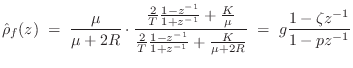
 (digital
  (digital zero)
The transmittance filter is again
Feathering
Since the pluck model is linear, the parameters are not signal-dependent. As a result, when the string and spring separate, there is a discontinuous change in the reflection and transmission coefficients. In practice, it is useful to ``feather'' the switch-over from one model to the next [470]. In this instance, one appealing choice is to introduce a nonlinear spring, as is commonly used for piano-hammer models (see §9.3.2 for details).
Let the nonlinear spring model take the form
The foregoing suggests a nonlinear tapering of the damping ![]() in
addition to the tapering the stiffness
in
addition to the tapering the stiffness ![]() as the spring compression
approaches zero. One natural choice would be
as the spring compression
approaches zero. One natural choice would be
In summary, the engagement and disengagement of the plucking system can be ``feathered'' by a nonlinear spring and damper in the plectrum model.
Piano Synthesis
The main elements of the piano we need to model are the
- hammer (§9.3.2),
- string (Chapter 6, §6.6),
- bridge (§9.2.1), and
- soundboard, enclosure, acoustic space, mic placement, etc.
From the bridge (which runs along the soundboard) to each ``virtual microphone'' (or ``virtual ear''), the soundboard, enclosure, and listening space can be well modeled as a high-order LTI filter characterized by its impulse response (Chapter 8). Such long impulse responses can be converted to more efficient recursive digital filters by various means (Chapter 3,§8.6.2).
A straightforward piano model along the lines indicated above turns out to be relatively expensive computationally. Therefore, we also discuss, in §9.4.4 below, the more specialized commuted piano synthesis technique [467], which is capable of high quality piano synthesis at low cost relative to other model-based approaches. It can be seen as a hybrid method in which the string is physically modeled, the hammer is represented by a signal model, and the acoustic resonators (soundboard, enclosure, etc.) are handled by ordinary sampling (of their impulse response).
Stiff Piano Strings
Piano strings are audibly inharmonic due to stiffness [211,210]. General stiff-string modeling was introduced in §6.9. In this section, we discuss further details specific to piano strings.
The main effect of string stiffness is to stretch the partial overtone series, so that piano tones are not precisely harmonic [144]. As a result, piano tuners typically stretch the tuning of the piano slightly. For example, the total amount of tuning stretch from the lowest to highest note has been measured to be approximately 35 cents on a Kurzweil PC88, 45 cents on a Steinway Model M, and 60 cents on a Steinway Model D.10.17
Piano String Wave Equation
A wave equation suitable for modeling linearized piano strings is given by [77,45,317,517]
where the partial derivative notation
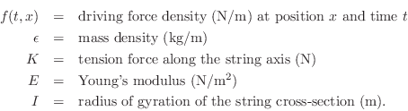
Young's modulus and the radius of gyration are defined in Appendix B.
The first two terms on the right-hand side of Eq.![]() (9.30) come from
the ideal string wave equation (see Eq.
(9.30) come from
the ideal string wave equation (see Eq.![]() (C.1)), and they model
transverse acceleration and transverse restoring force due to tension,
respectively. The term
(C.1)), and they model
transverse acceleration and transverse restoring force due to tension,
respectively. The term ![]() approximates the transverse
restoring force exerted by a stiff string when it is bent. In an
ideal string with zero diameter, this force is zero; in an ideal
rod (or bar), this term is dominant [317,261,169].
The final two terms provide damping. The damping associated
with
approximates the transverse
restoring force exerted by a stiff string when it is bent. In an
ideal string with zero diameter, this force is zero; in an ideal
rod (or bar), this term is dominant [317,261,169].
The final two terms provide damping. The damping associated
with ![]() is frequency-independent, while the damping due
is frequency-independent, while the damping due ![]() increases with frequency.
increases with frequency.
Damping-Filter Design
In [46], the damping in real piano strings was modeled using a length 17 FIR filter for the lowest strings, and a length 9 FIR filter for the remaining strings. Such FIR filters (or nonparametric measured frequency-response data) can be converted to lower-order IIR filters by the usual methods (§8.6.2). It is convenient to have separate damping and dispersion filters in the string model. The damping filter in piano strings is significantly less demanding than the dispersion filter.
Dispersion Filter-Design
In the context of a digital waveguide string model, dispersion associated with stiff strings can be supplied by an allpass filter in the basic feedback loop. Methods for designing dispersion allpass filters were summarized in §6.11.3. In this section, we are mainly concerned with how to specify the desired dispersion allpass filter for piano strings.
Perceptual studies regarding the audibility of inharmonicity in stringed instrument sounds [211] indicate that the just noticeable coefficient of inharmonicity is given approximately by
where
For a stiff string with Young's modulus
where
In general, when designing dispersion filters for vibrating string models, it is highly cost-effective to obtain an allpass filter which correctly tunes only the lowest-frequency partial overtones, where the number of partials correctly tuned is significantly less than the total number of partials present, as in [384].
Application of the method of [2] to piano-string dispersion-filter design is reported in [1].
A Faust implementation of a closed-form expression
[367] for dispersion allpass coefficients as a
function of inharmonicity coefficient ![]() may be found in the function
piano_dispersion_filter within effect.lib.
may be found in the function
piano_dispersion_filter within effect.lib.
Nonlinear Piano Strings
It turns out that piano strings exhibit audible nonlinear effects,
especially in the first three octaves of its pitch range at fortissimo
playing levels and beyond [26]. As a result, for
highest quality piano synthesis, we need more than what is obtainable
from a linearized wave equation such as Eq.![]() (9.30).
(9.30).
As can be seen from a derivation of the wave equation for an ideal
string vibrating in 3D space (§B.6), there is
fundamentally nonlinear coupling between transverse and
longitudinal string vibrations. It turns out that the coupling from
transverse-to-longitudinal is much stronger than vice versa, so that
piano synthesis models can get by with one-way coupling at normal
dynamic playing levels [30,163]. As
elaborated in §B.6 and the references cited there, the
longitudinal displacement ![]() is driven by longitudinal changes in the
squared slope of the string:
is driven by longitudinal changes in the
squared slope of the string:
![$\displaystyle [(y')^2]' \isdefs \frac{\partial}{\partial x} \left[\frac{\partial}{\partial x}\, y(t,x)\right]^2.
$](http://www.dsprelated.com/josimages_new/pasp/img2270.png)
In addition to the excitation of longitudinal modes, the nonlinear transverse-to-longitudinal coupling results in a powerful longitudinal attack pulse, which is the leading component of the initial ``shock noise'' audible in a piano tone. This longitudinal attack pulse hits the bridge well before the first transverse wave and is therefore quite significant perceptually. A detailed simulation of both longitudinal and transverse waves in an ideal string excited by a Gaussian pulse is given in [391].
Another important (i.e., audible) effect due to nonlinear transverse-to-longitudinal coupling is so-called phantom partials. Phantom partials are ongoing intermodulation products from the transverse partials as they transduce (nonlinearly) into longitudinal waves. The term ``phantom partial'' was coined by Conklin [85]. The Web version of [18] includes some illuminating sound examples by Conklin.
Nonlinear Piano-String Synthesis
When one-way transverse-to-longitudinal coupling is sufficiently accurate, we can model its effects separately based on observations of transverse waves. For example [30,28],
- longitudinal modes can be implemented as second-order
resonators (``modal synthesis''), with driving coefficients
given by
- orthogonally projecting [451] the spatial
derivative of the squared string slope onto the longitudinal mode
shapes (both functions of position
 ).
).
- If tension variations along the string are neglected (reasonable
since longitudinal waves are so much faster than transverse waves),
then the longitudinal force on the bridge can be derived from the
estimated instantaneous tension in the string, and efficient
methods for this have been developed for guitar-string synthesis,
particularly by Tolonen (§9.1.6).
An excellent review of nonlinear piano-string synthesis (emphasizing the modal synthesis approach) is given in [30].
Regimes of Piano-String Vibration
In general, more complex synthesis models are needed at higher dynamic playing levels. The main three regimes of vibration are as follows [27]:
- The simplest piano-string vibration regime is characterized by
linear superposition in which transverse and longitudinal
waves decouple into separate modes, as implied by
Eq.
 (9.30). In this case, transverse and longitudinal waves can
be simulated in separate digital waveguides (Ch. 6).
The longitudinal waveguide is of course an order of magnitude
shorter than the transverse waveguide(s).
(9.30). In this case, transverse and longitudinal waves can
be simulated in separate digital waveguides (Ch. 6).
The longitudinal waveguide is of course an order of magnitude
shorter than the transverse waveguide(s).
- As dynamic playing level is increased,
transverse-to-longitudinal coupling becomes audible
[26].
- At very high dynamic levels, the model should also include
longitudinal-to-transverse coupling. However, this is usually
neglected.
Efficient Waveguide Synthesis of Nonlinear Piano Strings
The following nonlinear waveguide piano-synthesis model is under current consideration [427]:
- Initial striking force determines the starting regime (1, 2, or 3 above).
- The string model is simplified as it decays.
Because the energy stored in a piano string decays monotonically after
a hammer strike (neglecting coupling from other strings), we may
switch to progressively simpler models as the energy of
vibration falls below corresponding thresholds. Since the purpose of
model-switching is merely to save computation, it need not happen
immediately, so it may be triggered by a string-energy estimate based
on observing the string at a single point ![]() over the past
period or so of vibration. Perhaps most simply, the model-regime
classifier can be based on the maximum magnitude of the bridge
force over at least one period. If the regime 2 model includes an
instantaneous string-length (tension) estimate, one may simply compare
that to a threshold to determine when the simpler model can be used.
If the longitudinal components and/or phantom partials are not
completely inaudible when the model switches, then standard
cross-fading techniques should be applied so that inharmonic partials
are faded out rather than abruptly and audibly cut off.
over the past
period or so of vibration. Perhaps most simply, the model-regime
classifier can be based on the maximum magnitude of the bridge
force over at least one period. If the regime 2 model includes an
instantaneous string-length (tension) estimate, one may simply compare
that to a threshold to determine when the simpler model can be used.
If the longitudinal components and/or phantom partials are not
completely inaudible when the model switches, then standard
cross-fading techniques should be applied so that inharmonic partials
are faded out rather than abruptly and audibly cut off.
To obtain a realistic initial shock noise in the tone for regime 1 (and for any model that does not compute it automatically), the appropriate shock pulse, computed as a function of hammer striking force (or velocity, displacement, etc.), can be summed into the longitudinal waveguide during the hammer contact period.
The longitudinal bridge force may be generated from the estimated string length (§9.1.6). This force should be exerted on the bridge in the direction coaxial with the string at the bridge (a direction available from the two transverse displacements one sample away from the bridge).
Phantom partials may be generated in the longitudinal waveguide as explicit intermodulation products based on the transverse-wave overtones known to be most contributing; for example, the Goetzel algorithm [451] could be used to track relevant partial amplitudes for this purpose. Such explicit synthesis of phantom partials, however, makes modal synthesis more compelling for the longitudinal component [30]; in a modal synthesis model, the longitudinal attack pulse can be replaced by a one-shot (per hammer strike) table playback, scaled and perhaps filtered as a function of the hammer striking velocity.
On the high end for regime 2 modeling, a full nonlinear coupling may be implemented along the three waveguides (two transverse and one longitudinal). At this level of complexity, a wide variety of finite-difference schemes should also be considered (§7.3.1) [53,555].
Checking the Approximations
The preceding discussion considered several possible approximations for nonlinear piano-string synthesis. Other neglected terms in the stiff-string wave equation were not even discussed, such as terms due to shear deformation and rotary inertia that are included in the (highly accurate) Timoshenko beam theory formulation [261,169]. The following questions naturally arise:
- How do we know for sure our approximations are inaudible?
- We can listen, but could we miss an audible effect?
- Could a difference become audible after more listening?
Note that there are software tools (e.g., from the world of perceptual audio coding [62,472]) that can be used to measure the audible equivalence of two sounds [456]. For an audio coder, these tools predict the audibility of the difference between original and compressed sounds. For sound synthesis applications, we want to compare our ``exact'' and ``computationally efficient'' synthesis models.
High-Accuracy Piano-String Modeling
In [265,266], an extension of the mass-spring model of [391] was presented for the purpose of high-accuracy modeling of nonlinear piano strings struck by a hammer model such as described in §9.3.2. This section provides a brief overview.
![\includegraphics[width=0.35\twidth]{eps/massspringmass}](http://www.dsprelated.com/josimages_new/pasp/img2271.png)
Figure 9.25 shows a mass-spring model in 3D space. From Hooke's Law (§B.1.3), we have
![\begin{eqnarray*}
m_1\, \underline{{\ddot x}}_1 \eqsp \underline{f}_1
&=& k\cdo...
...,\right\Vert}\right]\left(\underline{x}_2-\underline{x}_1\right)
\end{eqnarray*}](http://www.dsprelated.com/josimages_new/pasp/img2276.png)
and similarly for mass 2, where
![]() is the vector
position of mass
is the vector
position of mass ![]() in 3D space.
in 3D space.
Generalizing to a chain of masses and spring is shown in Fig.9.26. Mass-spring chains--also called beaded strings--have been analyzed in numerous textbooks (e.g., [295,318]), and numerical software simulation is described in [391].
![\includegraphics[width=0.8\twidth]{eps/massspringstring}](http://www.dsprelated.com/josimages_new/pasp/img2278.png)
The force on the ![]() th mass can be expressed as
th mass can be expressed as
where
![$\displaystyle \alpha_i \isdefs k\cdot \left[1-\frac{l_0}{\left\Vert\,\underline{x}_{i+1}-\underline{x}_i\,\right\Vert}\right].
$](http://www.dsprelated.com/josimages_new/pasp/img2282.png)
A Stiff Mass-Spring String Model
Following the classical derivation of the stiff-string wave equation [317,144], an obvious way to introduce stiffness in the mass-spring chain is to use a bundle of mass-spring chains to form a kind of ``lumped stranded cable''. One section of such a model is shown in Fig.9.27. Each mass is now modeled as a 2D mass disk. Complicated rotational dynamics can be avoided by assuming no torsional waves (no ``twisting'' motion) (§B.4.20).
A three-spring-per-mass model is shown in Fig.9.28
[266]. The spring positions alternate between angles
![]() , say, on one side of a mass disk and
, say, on one side of a mass disk and
![]() on the other side in order to provide effectively
six spring-connection points around the mass disk for only
three connecting springs per section. This improves isotropy
of the string model with respect to bending direction.
on the other side in order to provide effectively
six spring-connection points around the mass disk for only
three connecting springs per section. This improves isotropy
of the string model with respect to bending direction.
![\includegraphics[width=0.8\twidth]{eps/masssprings3circ}](http://www.dsprelated.com/josimages_new/pasp/img2286.png)
A problem with the simple mass-spring-chain-bundle is that there is no
resistance whatsoever to shear deformation, as is clear from
Fig.9.29. To rectify this problem (which does not
arise due implicit assumptions when classically deriving the
stiff-string wave equation), diagonal springs can be added to the
model, as shown in
Fig.![]() .
.
In the simulation results reported in [266], the spring-constants of the shear springs were chosen so that their stiffness in the longitudinal direction would equal that of the longitudinal springs.
![\includegraphics[width=0.4\twidth]{eps/masssprings3shear}](http://www.dsprelated.com/josimages_new/pasp/img2288.png)
Nonlinear Piano-String Equations of Motion in State-Space Form
For the flexible (non-stiff) mass-spring string, referring to
Fig.9.26 and Eq.![]() (9.34), we have the following
equations of motion:
(9.34), we have the following
equations of motion:
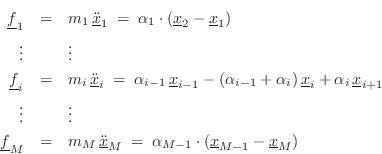
or, in ![]() vector form,
vector form,
Finite Difference Implementation
Digitizing
![]() via the centered second-order difference
[Eq.
via the centered second-order difference
[Eq.![]() (7.5)]
(7.5)]
Note that requiring three adjacent spatial string samples to be in
contact with the piano hammer during the attack (which helps to
suppress aliasing of spatial frequencies on the string during the
attack) implies a sampling rate in the vicinity of 6 megahertz
[265]. Thus, the model is expensive to compute!
However, results to date show a high degree of accuracy, as desired.
In particular, the stretching of the partial overtones in the
stiff-string model of
Fig.![]() has
been measured to be highly accurate despite using only three spring
attachment points on one side of each mass disk [265].
has
been measured to be highly accurate despite using only three spring
attachment points on one side of each mass disk [265].
See [53] for alternative finite-difference formulations that better preserve physical energy and have other nice properties worth considering.
Commuted Piano Synthesis
The general technique of commuted synthesis was introduced in §8.7. This method is enabled by the linearity and time invariance of both the vibrating string and its acoustic resonator, allowing them to be interchanged, in principle, without altering the overall transfer function [449].
While the piano-hammer is a strongly nonlinear element (§9.3.2),
it is nevertheless possible to synthesize a piano using commuted
synthesis with high fidelity and low computational cost given the
approximation that the string itself is linear and time-invariant
(§9.4.2) [467,519,30].
The key observation is that the interaction
between the hammer and string is essentially discrete (after
deconvolution) at only one or a few time instants per hammer strike.
The deconvolution needed is a function of the hammer-string collision
velocity ![]() . As a result, the hammer-string interaction can
be modeled as one or a few discrete impulses that are filtered in a
. As a result, the hammer-string interaction can
be modeled as one or a few discrete impulses that are filtered in a
![]() -dependent way.
-dependent way.
Figure 9.31 illustrates a typical series of interaction forces-pulses at the contact point between a piano-hammer and string. The vertical lines indicate the locations and amplitudes of three single-sample impulses passed through three single-pulse filters to produce the overlapping pulses shown.
![\includegraphics[width=0.6\twidth]{eps/pianoForcePulses}](http://www.dsprelated.com/josimages_new/pasp/img2298.png)
Force-Pulse Synthesis
![\includegraphics[width=0.95\twidth]{eps/pianoForcePulse}](http://www.dsprelated.com/josimages_new/pasp/img2299.png) |
The creation of a single force-pulse for a given hammer-string
collision velocity ![]() (a specific ``dynamic level'') is shown in
Fig.9.32. The filter input is an impulse, and the
output is the desired hammer-string force pulse. As
(a specific ``dynamic level'') is shown in
Fig.9.32. The filter input is an impulse, and the
output is the desired hammer-string force pulse. As ![]() increases,
the output pulse increases in amplitude and decreases in width,
which means the filter is nonlinear. In other words, the force pulse
gets ``brighter'' as its amplitude (dynamic level) increases. In a
real piano, this brightness increase is caused by the nonlinear
felt-compression in the piano hammer. Recall from §9.3.2
that piano-hammer felt is typically modeled as a nonlinear spring
described by
increases,
the output pulse increases in amplitude and decreases in width,
which means the filter is nonlinear. In other words, the force pulse
gets ``brighter'' as its amplitude (dynamic level) increases. In a
real piano, this brightness increase is caused by the nonlinear
felt-compression in the piano hammer. Recall from §9.3.2
that piano-hammer felt is typically modeled as a nonlinear spring
described by
![]() , where
, where ![]() is felt compression. Here, the
brightness is increased by shrinking the duration of the filter
impulse response as
is felt compression. Here, the
brightness is increased by shrinking the duration of the filter
impulse response as ![]() increases. The key property enabling
commuted synthesis is that, when
increases. The key property enabling
commuted synthesis is that, when ![]() is constant, the filter
operates as a normal LTI filter. In this way, the entire piano has
been ``linearized'' with respect to a given collision velocity
is constant, the filter
operates as a normal LTI filter. In this way, the entire piano has
been ``linearized'' with respect to a given collision velocity ![]() .
.
Multiple Force-Pulse Synthesis
One method of generating multiple force pulses as shown in
Fig.9.31 is to sum several single-pulse filters, as
shown in Fig.9.33. Furthermore, the three input
impulses can be generated using a single impulse into a tapped delay
line (§2.5). The sum of the three filter outputs gives the
desired superposition of three hammer-string force pulses. As the
collision velocity ![]() increases, the output pulses become taller
and thinner, showing less overlap. The filters LPF1-LPF3 can be
given
increases, the output pulses become taller
and thinner, showing less overlap. The filters LPF1-LPF3 can be
given ![]() as side information, or the input impulse amplitudes can
be set to
as side information, or the input impulse amplitudes can
be set to ![]() , or the like.
, or the like.
![\includegraphics[width=\twidth]{eps/pianoForceFilterPulses}](http://www.dsprelated.com/josimages_new/pasp/img2301.png) |
Commuted Piano Synthesis Architecture
Figure 9.34 shows a complete piano synthesis system along the lines discussed. At a fixed dynamic level, we have the critical feature that the model is linear and time invariant. Therefore we may commute the ``Soundboard & Enclosure'' filter with not only the string, but with the hammer filter-bank as well. The result is shown in Fig.9.35.
![\includegraphics[width=\twidth]{eps/pianoCommutedA}](http://www.dsprelated.com/josimages_new/pasp/img2302.png)
![\includegraphics[width=\twidth]{eps/pianoCommutedB}](http://www.dsprelated.com/josimages_new/pasp/img2303.png)
As in the case of commuted guitar synthesis (§8.7), we replace a high-order digital filter (at least thousands of poles and zeros [229]) with a simple excitation table containing that filter's impulse response. Thus, the large digital filter required to implement the soundboard, piano enclosure, and surrounding acoustic space, has been eliminated. At the same time, we still have explicit models for the hammer and string, so physical variations can be implemented, such as harder or softer hammers, more or less string stiffness, and so on.
Even some resonator modifications remain possible, however, such as changing the virtual mic positions (§2.2.7). However, if we now want to ``open the top'' of our virtual piano, we have to measure the impulse response that case separately and have a separate table for it, which is not a problem, but it means we're doing ``sampling'' instead of ``modeling'' of the various resonators.
An approximation made in the commuted technique is that detailed reflections generated on the string during hammer-string contact are neglected; that is, the hammer force-pulse depends only on the hammer-string velocity at the time of their initial contact, and the string velocity is treated as remaining constant throughout the contact duration.
Progressive Filtering
To save computation in the filtering, we can make use of the observation that, under the assumption of a string initially at rest, each interaction pulse is smoother than the one before it. That suggests applying the force-pulse filtering progressively, as was done with Leslie cabinet reflections in §5.7.6. In other words, the second force-pulse is generated as a filtering of the first force-pulse. This arrangement is shown in Fig.9.36.
![\includegraphics[width=\twidth]{eps/pianoThreeDelayedFilters}](http://www.dsprelated.com/josimages_new/pasp/img2304.png) |
With progressive filtering, each filter need only supply the mild smoothing (and perhaps dispersion) associated with traveling from the hammer to the agraffe and back, plus the mild attenuation associated with reflection from the felt-covered hammer (a nonlinear mass-spring system as described in §9.3.2).
Referring to Fig.9.36, The first filter LPF1 can shape a velocity-independent excitation signal to obtain the appropriate ``shock spectrum'' for that hammer velocity. Alternatively, the Excitation Table itself can be varied with velocity to produce the needed signal. In this case, filter LPF1 can be eliminated entirely by applying it in advance to the excitation signal. It is possible to interpolate between tables for two different striking velocities; in this case, the tables should be pre-processed to eliminate phase cancellations during cross-fade.
Assuming the first filter in Fig.9.36 is
``weakest'' at the highest hammer velocity (MIDI velocity ![]() ), that
filtering can be applied to the excitation table in advance, and the first
filter then becomes no computation for MIDI velocity
), that
filtering can be applied to the excitation table in advance, and the first
filter then becomes no computation for MIDI velocity ![]() , and as velocity
is lowered, the filter only needs to make up the difference between what
was done in advance to the table and what is desired at that velocity.
, and as velocity
is lowered, the filter only needs to make up the difference between what
was done in advance to the table and what is desired at that velocity.
Since, for most keys, only a few interaction impulses are observed, per hammer strike, in real pianos, this computational model of the piano achieves a high degree of realism for a price comparable to the cost of the strings only. The soundboard and enclosure filtering have been eliminated and replaced by a look-up table using a few read-pointers per note, and the hammer costs only one or a few low-order filters which in principle convert the interaction impulse into an accurate force pulse.
Excitation Factoring
As another refinement, it is typically more efficient to implement the highest Q resonances of the soundboard and piano enclosure using actual digital filters (see §8.8). By factoring these out, the impulse response is shortened and thus the required excitable length is reduced. This provides a classical computation vs. memory trade-off which can be optimized as needed in a given implementation. For lack of a better name, let us refer to such a resonator bank as an ``equalizer'' since it can be conveniently implemented using parametric equalizer sections, one per high-Q resonance.
A possible placement of the comb filter and equalizer is shown in Fig.9.37. The resonator/eq/reverb/comb-filter block may include filtering for partially implementing the response of the soundboard and enclosure, equalization sections for piano color variations, reverberation, comb-filter(s) for flanging, chorus, and simulated hammer-strike echoes on the string. Multiple outputs having different spectral characteristics can be extracted at various points in the processing.
![\includegraphics[scale=0.9]{eps/pianoComplete}](http://www.dsprelated.com/josimages_new/pasp/img2306.png)
Excitation Synthesis
For a further reduction in cost of implementation, particularly with respect to memory usage, it is possible to synthesize the excitation using a noise signal through a time-varying lowpass filter [440]. The synthesis replaces the recorded soundbard/enclosure sound. It turns out that the sound produced by tapping on a piano soundboard sounds very similar to noise which is lowpass-filtered such that the filter bandwidth contracts over time. This approach is especially effective when applied only to the high-frequency residual excitation after factoring out all long-ringing modes as biquads.
Coupled Piano Strings
Perhaps it should be emphasized that for good string-tone synthesis, multiple filtered delay loops should be employed for each note rather than the single-loop case so often used for simplicity (§6.12; §C.13). For piano, two or three delay loops can correspond to the two or three strings hit by the same hammer in the plane orthogonal to both the string and bridge. This number of delay loops is doubled from there if the transverse vibration planes parallel to the bridge are added; since these are slightly detuned, they are worth considering. Finally, another 2-3 (shorter) delay loops are needed to incorporate longitudinal waves for each string, and all loops should be appropriately coupled. In fact, for full accurancy, longitudinal waves and transverse waves should be nonlinearly coupled along the length of the string [391] (see §B.6.2).
Commuted Synthesis of String Reverberation
The sound of all strings ringing can be summed with the excitation to simulate the effect of many strings resonating with the played string when the sustain pedal is down [519]. The string loop filters out the unwanted frequencies in this signal and selects only the overtones which would be excited by the played string.
High Piano Key Numbers
At very high pitches, the delay-line length used in the string may become too short for the implementation used, especially when using vectorized module signals (sometimes called ``chunks'' in place of samples [355]). In this case, good results can be obtained by replacing the filtered-delay-loop string model by a simpler model consisting only of a few parallel, second-order filter sections or enveloped sinusoidal oscillators, etc. In other words, modal synthesis (§8.5) is a good choice for very high key numbers.
Force-Pulse Filter Design
In the commuted piano synthesis technique, it is necessary to fit a
filter impulse response to the desired hammer-string force-pulse shape
for each key and for each key velocity ![]() , as
indicated in Figures 9.32 and 9.33. Such a
desired curve can be found in the musical acoustics literature
[488] or it can be easily generated from a good piano-hammer
model (§9.3.2) striking the chosen piano string model.
, as
indicated in Figures 9.32 and 9.33. Such a
desired curve can be found in the musical acoustics literature
[488] or it can be easily generated from a good piano-hammer
model (§9.3.2) striking the chosen piano string model.
For psychoacoustic reasons, it is preferable to optimize the force-pulse filter-coefficients in the frequency domain §8.6.2. Some additional suggestions are given in [467,519].
Literature on Piano Acoustics and Synthesis
There has been much research into the musical acoustics of the piano, including models of piano strings [543,18,75,76,144,42] and the piano hammer [493,63,178,60,486,164,487]. Additionally, there has been considerable work to date on the problem of piano synthesis by digital waveguide methods [467,519,523,56,42].
A careful computational model of the piano, partially based on physical modeling and suitable for high-quality real-time sound synthesis, was developed by Bensa in the context of his thesis work [42]. Related publications include [43,45,46].
An excellent simulation of the clavichord, also using the commuted waveguide synthesis technique, is described in [501]. A detailed simulation of the harpsichord, along similar lines, but with some interesting new variations, may be found in [514].
The 2003 paper of Bank et al. [29] includes good summaries of prior research on elements of piano modeling such as efficient computational string models, loss-filter design, dispersion filter design, and soundboard models. A more recent paper in this area is [30].
Woodwinds
We now consider models of woodwind instruments, focusing on the single-reed case. In §9.5.4, tonehole modeling is described in some detail.
Single-Reed Instruments
A simplified model for a single-reed woodwind instrument is shown in Fig. 9.38 [431].
![\includegraphics[width=\twidth]{eps/fSingleReedAI}](http://www.dsprelated.com/josimages_new/pasp/img2307.png)
If the bore is cylindrical, as in the clarinet, it can be modeled quite simply using a bidirectional delay line. If the bore is conical, such as in a saxophone, it can still be modeled as a bidirectional delay line, but interfacing to it is slightly more complex, especially at the mouthpiece [37,7,160,436,506,507,502,526,406,528], Because the main control variable for the instrument is air pressure in the mouth at the reed, it is convenient to choose pressure wave variables.
To first order, the bell passes high frequencies and reflects low
frequencies, where ``high'' and ``low'' frequencies are divided by the
wavelength which equals the bell's diameter. Thus, the bell can be regarded
as a simple ``cross-over'' network, as is used to split signal energy
between a woofer and tweeter in a loudspeaker cabinet. For a clarinet
bore, the nominal ``cross-over frequency'' is around ![]() Hz
[38]. The flare of the bell lowers the cross-over frequency by
decreasing the bore characteristic impedance toward the end in an
approximately non-reflecting manner [51]. Bell flare can
therefore be
considered analogous to a transmission-line transformer.
Hz
[38]. The flare of the bell lowers the cross-over frequency by
decreasing the bore characteristic impedance toward the end in an
approximately non-reflecting manner [51]. Bell flare can
therefore be
considered analogous to a transmission-line transformer.
Since the length of the clarinet bore is only a quarter wavelength at the fundamental frequency, (in the lowest, or ``chalumeau'' register), and since the bell diameter is much smaller than the bore length, most of the sound energy traveling into the bell reflects back into the bore. The low-frequency energy that makes it out of the bore radiates in a fairly omnidirectional pattern. Very high-frequency traveling waves do not ``see'' the enclosing bell and pass right through it, radiating in a more directional beam. The directionality of the beam is proportional to how many wavelengths fit along the bell diameter; in fact, many wavelengths away from the bell, the radiation pattern is proportional to the two-dimensional spatial Fourier transform of the exit aperture (a disk at the end of the bell) [308].
The theory of the single reed is described, e.g., in [102,249,308]. In the digital waveguide clarinet model described below [431], the reed is modeled as a signal- and embouchure-dependent nonlinear reflection coefficient terminating the bore. Such a model is possible because the reed mass is neglected. The player's embouchure controls damping of the reed, reed aperture width, and other parameters, and these can be implemented as parameters on the contents of the lookup table or nonlinear function.
Digital Waveguide Single-Reed Implementation
A diagram of the basic clarinet model is shown in
Fig.9.39. The delay-lines carry left-going and
right-going pressure samples ![]() and
and ![]() (respectively) which
sample the traveling pressure-wave components within the bore.
(respectively) which
sample the traveling pressure-wave components within the bore.
![\includegraphics[width=\twidth]{eps/fSingleReedWGM}](http://www.dsprelated.com/josimages_new/pasp/img2311.png)
The reflection filter at the right implements the bell or tone-hole
losses as well as the round-trip attenuation losses from traveling
back and forth in the bore. The bell output filter is highpass, and
power complementary with respect to the bell reflection filter
[500]. Power complementarity follows from the
assumption that the bell itself does not vibrate or otherwise absorb
sound. The bell is also amplitude complementary. As a result,
given a reflection filter ![]() designed to match measured mode
decay-rates in the bore, the transmission filter can be written down
simply as
designed to match measured mode
decay-rates in the bore, the transmission filter can be written down
simply as
![]() for velocity waves, or
for velocity waves, or
![]() for pressure waves. It is easy to show that such
amplitude-complementary filters are also power complementary by
summing the transmitted and reflected power waves:
for pressure waves. It is easy to show that such
amplitude-complementary filters are also power complementary by
summing the transmitted and reflected power waves:
![\begin{eqnarray*}
P_t U_t + P_r U_r &=& (1+H_r)P \cdot (1-H_r)U + H_r P \cdot (-H_r)(-U)\\
&=& [1-H_r^2 + H_r^2]PU \;=\; PU,
\end{eqnarray*}](http://www.dsprelated.com/josimages_new/pasp/img2315.png)
where ![]() denotes the z transform transform of the incident pressure wave,
and
denotes the z transform transform of the incident pressure wave,
and ![]() denotes the z transform of the incident volume-velocity. (All
z transform have omitted arguments
denotes the z transform of the incident volume-velocity. (All
z transform have omitted arguments
![]() , where
, where
![]() denotes the sampling interval in seconds.)
denotes the sampling interval in seconds.)
At the far left is the reed mouthpiece controlled by mouth
pressure ![]() . Another control is embouchure, changed in
general by modifying the reflection-coefficient function
. Another control is embouchure, changed in
general by modifying the reflection-coefficient function
![]() , where
, where
![]() . A simple choice of embouchure control is an
offset in the reed-table address. Since the main feature of the reed table
is the pressure-drop where the reed begins to open, a simple embouchure
offset can implement the effect of biting harder or softer on the reed, or
changing the reed stiffness.
. A simple choice of embouchure control is an
offset in the reed-table address. Since the main feature of the reed table
is the pressure-drop where the reed begins to open, a simple embouchure
offset can implement the effect of biting harder or softer on the reed, or
changing the reed stiffness.
A View of Single-Reed Oscillation
To start the oscillation, the player applies a pressure at the mouthpiece which ``biases'' the reed in a ``negative-resistance'' region. (The pressure drop across the reed tends to close the air gap at the tip of the reed so that an increase in pressure will result in a net decrease in volume velocity--this is negative resistance.) The high-pressure front travels down the bore at the speed of sound until it encounters an open air hole or the bell. To a first approximation, the high-pressure wave reflects with a sign inversion and travels back up the bore. (In reality a lowpass filtering accompanies the reflection, and the complementary highpass filter shapes the spectrum that emanates away from the bore.)
As the negated pressure wave travels back up the bore, it cancels the elevated pressure that was established by the passage of the first wave. When the negated pressure front gets back to the mouthpiece, it is reflected again, this time with no sign inversion (because the mouthpiece looks like a closed end to a first approximation). Therefore, as the wave travels back down to the bore, a negative pressure zone is left behind. Reflecting from the open end again with a sign inversion brings a return-to-zero wave traveling back to the mouthpiece. Finally the positive traveling wave reaches the mouthpiece and starts the second ``period'' of oscillation, after four trips along the bore.
So far, we have produced oscillation without making any use of the negative-resistance of the reed aperture. This is merely the start-up transient. Since in reality there are places of pressure loss in the bore, some mechanism is needed to feed energy back into the bore and prevent the oscillation just described from decaying exponentially to zero. This is the function of the reed: When a traveling pressure-drop reflects from the mouthpiece, making pressure at the mouthpiece switch from high to low, the reed changes from open to closed (to first order). The closing of the reed increases the reflection coefficient ``seen'' by the impinging traveling wave, and so as the pressure falls, it is amplified by an increasing gain (whose maximum is unity when the reed shuts completely). This process sharpens the falling edge of the pressure drop. But this is not all. The closing of the reed also cuts back on the steady incoming flow from the mouth. This causes the pressure to drop even more, potentially providing effective amplification by more than unity.
An analogous story can be followed through for a rising pressure appearing at the mouthpiece. However, in the rising pressure case, the reflection coefficient falls as the pressure rises, resulting in a progressive attenuation of the reflected wave; however, the increased pressure let in from the mouth amplifies the reflecting wave. It turns out that the reflection of a positive wave is boosted when the incoming wave is below a certain level and it is attenuated above that level. When the oscillation reaches a very high amplitude, it is limited on the negative side by the shutting of the reed, which sets a maximum reflective amplification for the negative excursions, and it is limited on the positive side by the attenuation described above. Unlike classical negative-resistance oscillators, in which the negative-resistance device is terminated by a simple resistance instead of a lossy transmission line, a dynamic equilibrium is established between the amplification of the negative excursion and the dissipation of the positive excursion.
In the first-order case, where the reflection-coefficient varies linearly with pressure drop, it is easy to obtain an exact quantitative description of the entire process. In this case it can be shown, for example, that amplification occurs only on the positive half of the cycle, and the amplitude of oscillation is typically close to half the incoming mouth pressure (when losses in the bore are small). The threshold blowing pressure (which is relatively high in this simplified case) can also be computed in closed form.
Single-Reed Theory
![\includegraphics[scale=0.9]{eps/fReedSchematic}](http://www.dsprelated.com/josimages_new/pasp/img2321.png)
A simplified diagram of the clarinet mouthpiece is shown in
Fig. 9.40. The pressure in the mouth is assumed
to be a constant value ![]() , and the bore pressure
, and the bore pressure ![]() is defined
located at the mouthpiece. Any pressure drop
is defined
located at the mouthpiece. Any pressure drop
![]() across
the mouthpiece causes a flow
across
the mouthpiece causes a flow ![]() into the mouthpiece through the
reed-aperture impedance
into the mouthpiece through the
reed-aperture impedance
![]() which changes as a function of
which changes as a function of
![]() since the reed position is affected by
since the reed position is affected by
![]() . To a first
approximation, the clarinet reed can be regarded as a spring flap
regulated Bernoulli flow (§B.7.5), [249]).
This model has been verified well experimentally until the reed is
about to close, at which point viscosity effects begin to appear
[102]. It has also been verified that the mass
of the reed can be neglected to first order,10.18 so that
. To a first
approximation, the clarinet reed can be regarded as a spring flap
regulated Bernoulli flow (§B.7.5), [249]).
This model has been verified well experimentally until the reed is
about to close, at which point viscosity effects begin to appear
[102]. It has also been verified that the mass
of the reed can be neglected to first order,10.18 so that
![]() is a
positive real number for all values of
is a
positive real number for all values of
![]() . Possibly the most
important neglected phenomenon in this model is sound generation due
to turbulence of the flow, especially near reed closure. Practical
synthesis models have always included a noise component of some sort
which is modulated by the reed [431], despite a lack of firm
basis in acoustic measurements to date.
. Possibly the most
important neglected phenomenon in this model is sound generation due
to turbulence of the flow, especially near reed closure. Practical
synthesis models have always included a noise component of some sort
which is modulated by the reed [431], despite a lack of firm
basis in acoustic measurements to date.
The fundamental equation governing the action of the reed is continuity of volume velocity, i.e.,
where
and
is the volume velocity corresponding to the incoming pressure wave
In operation, the mouth pressure ![]() and incoming traveling bore pressure
and incoming traveling bore pressure
![]() are given, and the reed computation must produce an outgoing bore
pressure
are given, and the reed computation must produce an outgoing bore
pressure ![]() which satisfies (9.35), i.e., such that
which satisfies (9.35), i.e., such that
Solving for
It is helpful to normalize (9.38) as follows: Define
![]() , and note that
, and note that
![]() , where
, where
![]() . Then (9.38) can be multiplied through by
. Then (9.38) can be multiplied through by ![]() and
written as
and
written as
![]() , or
, or
The solution is obtained by plotting
| (10.40) |
An example of the qualitative appearance of ![]() overlaying
overlaying
![]() is shown in Fig. 9.41.
is shown in Fig. 9.41.
![\includegraphics[width=\twidth]{eps/fReedRelations}](http://www.dsprelated.com/josimages_new/pasp/img2346.png)
Scattering-Theoretic Formulation
Equation (9.38) can be solved for ![]() to obtain
to obtain

where
 |
(10.44) |
We interpret
Since the mouthpiece of a clarinet is nearly closed,
![]() which
implies
which
implies
![]() and
and
![]() . In the limit as
. In the limit as ![]() goes to
infinity relative to
goes to
infinity relative to ![]() , (9.42) reduces to the simple form of a
rigidly capped acoustic tube, i.e.,
, (9.42) reduces to the simple form of a
rigidly capped acoustic tube, i.e.,
![]() .
If it were possible to open the reed wide enough to achieve
matched impedance,
.
If it were possible to open the reed wide enough to achieve
matched impedance, ![]() , then we would have
, then we would have ![]() and
and ![]() , in
which case
, in
which case
![]() , with no reflection of
, with no reflection of ![]() , as expected. If
the mouthpiece is removed altogether to give
, as expected. If
the mouthpiece is removed altogether to give ![]() (regarding it now as a
tube section of infinite radius), then
(regarding it now as a
tube section of infinite radius), then ![]() ,
, ![]() , and
, and
![]() .
.
Computational Methods
Since finding the intersection of ![]() and
and
![]() requires an expensive
iterative algorithm with variable convergence times, it is not well suited
for real-time operation. In this section, fast algorithms based on
precomputed nonlinearities are described.
requires an expensive
iterative algorithm with variable convergence times, it is not well suited
for real-time operation. In this section, fast algorithms based on
precomputed nonlinearities are described.
Let ![]() denote half-pressure
denote half-pressure ![]() , i.e.,
, i.e.,
![]() and
and
![]() . Then (9.43) becomes
. Then (9.43) becomes
Subtracting this equation from
The last expression above can be used to precompute
| (10.47) |
(9.45) becomes
This is the form chosen for implementation in Fig. 9.39 [431]. The control variable is mouth half-pressure
Because the table contains a coefficient rather than a signal value, it
can be more heavily quantized both in address space and word length than
a direct lookup of a signal value such as
![]() or the like. A
direct signal lookup, though requiring much higher resolution, would
eliminate the multiplication associated with the scattering coefficient.
For example, if
or the like. A
direct signal lookup, though requiring much higher resolution, would
eliminate the multiplication associated with the scattering coefficient.
For example, if ![]() and
and ![]() are 16-bit signal samples,
the table would contain on the order of 64K 16-bit
are 16-bit signal samples,
the table would contain on the order of 64K 16-bit
![]() samples.
Clearly, some compression of this table would be desirable. Since
samples.
Clearly, some compression of this table would be desirable. Since
![]() is smoothly varying, significant compression is in fact
possible. However, because the table is directly in the signal path,
comparatively little compression can be done while maintaining full
audio quality (such as 16-bit accuracy).
is smoothly varying, significant compression is in fact
possible. However, because the table is directly in the signal path,
comparatively little compression can be done while maintaining full
audio quality (such as 16-bit accuracy).
![\includegraphics[width=4in]{eps/fReedTable}](http://www.dsprelated.com/josimages_new/pasp/img2382.png)
In the field of computer music, it is customary to use simple piecewise linear functions for functions other than signals at the audio sampling rate, e.g., for amplitude envelopes, FM-index functions, and so on [382,380]. Along these lines, good initial results were obtained [431] using the simplified qualitatively chosen reed table
depicted in Fig. 9.42 for
Another variation is to replace the table-lookup contents by a piecewise polynomial approximation. While less general, good results have been obtained in practice [89,91,92]. For example, one of the SynthBuilder [353] clarinet patches employs this technique using a cubic polynomial.
An intermediate approach between table lookups and polynomial approximations is to use interpolated table lookups. Typically, linear interpolation is used, but higher order polynomial interpolation can also be considered (see Chapter 4).
Clarinet Synthesis Implementation Details
To finish off the clarinet example, the remaining details of the SynthBuilder clarinet patch Clarinet2.sb are described.
The input mouth pressure is summed with a small amount of white noise,
corresponding to turbulence. For example, 0.1% is generally used as a
minimum, and larger amounts are appropriate during the attack of a note.
Ideally, the turbulence level should be computed automatically as a
function of pressure drop
![]() and reed opening geometry
[141,530]. It should also be lowpass filtered
as predicted by theory.
and reed opening geometry
[141,530]. It should also be lowpass filtered
as predicted by theory.
Referring to Fig. 9.39, the reflection filter is a simple one-pole with transfer function
 |
(10.50) |
where
Legato note transitions are managed using two delay line taps and cross-fading from one to the other during a transition [208,441,405]. In general, legato problems arise when the bore length is changed suddenly while sounding, corresponding to a new fingering. The reason is that really the model itself should be changed during a fingering change from that of a statically terminated bore to that of a bore with a new scattering junction appearing where each ``finger'' is lifting, and with disappearing scattering junctions where tone holes are being covered. In addition, if a hole is covered abruptly (especially when there are large mechanical caps, as in the saxophone), there will also be new signal energy injected in both directions on the bore in superposition with the signal scattering. As a result of this ideal picture, is difficult to get high quality legato performance using only a single delay line.
A reduced-cost, approximate solution for obtaining good sounding note transitions in a single delay-line model was proposed in [208]. In this technique, the bore delay line is ``branched'' during the transition, i.e., a second feedback loop is formed at the new loop delay, thus forming two delay lines sharing the same memory, one corresponding to the old pitch and the other corresponding to the new pitch. A cross-fade from the old-pitch delay to the new-pitch delay sounds good if the cross-fade time and duration are carefully chosen. Another way to look at this algorithm is in terms of ``read pointers'' and ``write pointers.'' A normal delay line consists of a single write pointer followed by a single read pointer, delayed by one period. During a legato transition, we simply cross-fade from a read-pointer at the old-pitch delay to a read-pointer at the new-pitch delay. In this type of implementation, the write-pointer always traverses the full delay memory corresponding to the minimum supported pitch in order that read-pointers may be instantiated at any pitch-period delay at any time. Conceptually, this simplified model of note transitions can be derived from the more rigorous model by replacing the tone-hole scattering junction by a single reflection coefficient.
STK software implementing a model as in Fig.9.39 can be found in the file Clarinet.cpp.
Tonehole Modeling
Toneholes in woodwind instruments are essentially cylindrical holes in
the bore. One modeling approach would be to treat the tonehole as a
small waveguide which connects to the main bore via one port on a
three-port junction. However, since the tonehole length is small
compared with the distance sound travels in one sampling instant (
![]() in, e.g.), it is more straightforward to treat the
tonehole as a lumped load along the bore, and most modeling efforts
have taken this approach.
in, e.g.), it is more straightforward to treat the
tonehole as a lumped load along the bore, and most modeling efforts
have taken this approach.
The musical acoustics literature contains experimentally verified models of tone-hole acoustics, such as by Keefe [238]. Keefe's tonehole model is formulated as a ``transmission matrix'' description, which we may convert to a traveling-wave formulation by a simple linear transformation (described in §9.5.4 below) [465]. For typical fingerings, the first few open tone holes jointly provide a bore termination [38]. Either the individual tone holes can be modeled as (interpolated) scattering junctions, or the whole ensemble of terminating tone holes can be modeled in aggregate using a single reflection and transmission filter, like the bell model. Since the tone hole diameters are small compared with most audio frequency wavelengths, the reflection and transmission coefficients can be implemented to a reasonable approximation as constants, as opposed to cross-over filters as in the bell. Taking into account the inertance of the air mass in the tone hole, the tone hole can be modeled as a two-port loaded junction having load impedance equal to the air-mass inertance [143,509]. At a higher level of accuracy, adapting transmission-matrix parameters from the existing musical acoustics literature leads to first-order reflection and transmission filters [238,406,403,404,465]. The individual tone-hole models can be simple lossy two-port junctions, modeling only the internal bore loss characteristics, or three-port junctions, modeling also the transmission characteristics to the outside air. Another approach to modeling toneholes is the ``wave digital'' model [527] (see §F.1 for a tutorial introduction to this approach). The subject of tone-hole modeling is elaborated further in [406,502]. For simplest practical implementation, the bell model can be used unchanged for all tunings, as if the bore were being cut to a new length for each note and the same bell were attached. However, for best results in dynamic performance, the tonehole model should additionally include an explicit valve model for physically accurate behavior when slowly opening or closing the tonehole [405].
The Clarinet Tonehole as a Two-Port Junction
![\includegraphics[scale=0.9]{eps/fFingerHoleKeefe}](http://www.dsprelated.com/josimages_new/pasp/img2398.png)
The clarinet tonehole model developed by Keefe [240] is
parametrized in terms of series and shunt resistance and reactance, as
shown in Fig. 9.43. The transmission
matrix description of this two-port is given by the product of the
transmission matrices for the series impedance ![]() , shunt
impedance
, shunt
impedance ![]() , and series impedance
, and series impedance ![]() , respectively:
, respectively:
![$\displaystyle \left[\begin{array}{c} P_1 \\ [2pt] U_1 \end{array}\right]$](http://www.dsprelated.com/josimages_new/pasp/img2401.png)
![$\displaystyle \left[\begin{array}{cc} 1 & R_a/2 \\ [2pt] 0 & 1 \end{array}\righ...
...1 \end{array}\right]
\left[\begin{array}{c} P_2 \\ [2pt] U_2 \end{array}\right]$](http://www.dsprelated.com/josimages_new/pasp/img2402.png)
![$\displaystyle \left[\begin{array}{cc} 1+\frac{R_a}{2R_s} & R_a[1+\frac{R_a}{4R_...
...} \end{array}\right]
\left[\begin{array}{c} P_2 \\ [2pt] U_2 \end{array}\right]$](http://www.dsprelated.com/josimages_new/pasp/img2403.png)
where all quantities are written in the frequency domain, and the impedance parameters are given by
| (open-hole shunt impedance) |
|||
| (closed-hole shunt impedance) |
(10.51) | ||
| (open-hole series impedance) |
|||
| (closed-hole series impedance) |
where
 |
|||
 |
where
![$\displaystyle t_h = t_w + \frac{1}{8}\frac{b^2}{a}\left[1+0.172\left(\frac{b}{a}\right)^2\right]
$](http://www.dsprelated.com/josimages_new/pasp/img2426.png)
Note that the specific resistance of the open tonehole, ![]() , is the
only real impedance and therefore the only source of wave energy loss at
the tonehole. It is given by [240]
, is the
only real impedance and therefore the only source of wave energy loss at
the tonehole. It is given by [240]

![$\displaystyle \alpha = \frac{1}{2bc}\left[\,\sqrt{\frac{2\eta\omega}{\rho}}
+ (\gamma-1)\sqrt{\frac{2\kappa\omega}{\rho C_p}}\,\right]
$](http://www.dsprelated.com/josimages_new/pasp/img2433.png)
where
The open-hole effective length ![]() , assuming no pad above the hole,
is given in
[240] as
, assuming no pad above the hole,
is given in
[240] as
![$\displaystyle t_e = \frac{(1/k)\tan(kt) + b [1.40 - 0.58(b/a)^2]}{1 - 0.61 kb \tan(kt)}
$](http://www.dsprelated.com/josimages_new/pasp/img2445.png)
For implementation in a digital waveguide model, the lumped parameters above must be converted to scattering parameters. Such formulations of toneholes have appeared in the literature: Vesa Välimäki [509,502] developed tonehole models based on a ``three-port'' digital waveguide junction loaded by an inertance, as described in Fletcher and Rossing [143], and also extended his results to the case of interpolated digital waveguides. It should be noted in this context, however, that in the terminology of Appendix C, Välimäki's tonehole representation is a loaded 2-port junction rather than a three-port junction. (A load can be considered formally equivalent to a ``waveguide'' having wave impedance given by the load impedance.) Scavone and Smith [402] developed digital waveguide tonehole models based on the more rigorous ``symmetric T'' acoustic model of Keefe [240], using general purpose digital filter design techniques to obtain rational approximations to the ideal tonehole frequency response. A detailed treatment appears in Scavone's CCRMA Ph.D. thesis [406]. This section, adapted from [465], considers an exact translation of the Keefe tonehole model, obtaining two one-filter implementations: the ``shared reflectance'' and ``shared transmittance'' forms. These forms are shown to be stable without introducing an approximation which neglects the series inertance terms in the tonehole model.
By substituting
![]() in (9.53) to convert spatial
frequency to temporal frequency, and by substituting
in (9.53) to convert spatial
frequency to temporal frequency, and by substituting
| (10.52) | |||
 |
(10.53) |
for
        Clear["t*", "p*", "u*", "r*"]
        transmissionMatrix = {{t11, t12}, {t21, t22}};
        leftPort = {{p2p+p2m}, {(p2p-p2m)/r2}};
        rightPort = {{p1p+p1m}, {(p1p-p1m)/r1}};
        Format[t11, TeXForm] := "{T_{11}}"
        Format[p1p, TeXForm] := "{P_1^+}"
        ... (etc. for all variables) ...
        TeXForm[Simplify[Solve[leftPort ==
               transmissionMatrix . rightPort, {p1m, p2p}]]]
The above code produces the following formulas:
Substituting relevant values for Keefe's tonehole model, we obtain, in matrix notation,
![$\displaystyle \left[\begin{array}{c} P_1^{-} \\ [2pt] P_2^{+} \end{array}\right]$](http://www.dsprelated.com/josimages_new/pasp/img2459.png)
![$\displaystyle \left[\begin{array}{cc} S & T \\ [2pt] T & S \end{array}\right]
\left[\begin{array}{c} P_1^{+} \\ [2pt] P_2^{-} \end{array}\right]$](http://www.dsprelated.com/josimages_new/pasp/img2460.png)
![$\displaystyle \quad
\left[\begin{array}{cc} 4R_aR_s + R_a^2 - 4R_0^2 & 8R_0R_s ...
...rray}\right]
\left[\begin{array}{c} P_1^{+} \\ [2pt] P_2^{-} \end{array}\right]$](http://www.dsprelated.com/josimages_new/pasp/img2462.png)
We thus obtain the scattering formulation depicted in Fig. 9.44, where
is the reflectance of the tonehole (the same from either direction), and
is the transmittance of the tonehole (also the same from either direction). The notation ``
![\includegraphics[scale=0.9]{eps/fFingerHoleScat}](http://www.dsprelated.com/josimages_new/pasp/img2465.png)
The approximate forms in (9.57) and (9.58) are obtained by neglecting
the negative series inertance ![]() which serves to adjust the effective
length of the bore, and which therefore can be implemented elsewhere in the
interpolated delay-line calculation as discussed further below. The open
and closed tonehole cases are obtained by substituting
which serves to adjust the effective
length of the bore, and which therefore can be implemented elsewhere in the
interpolated delay-line calculation as discussed further below. The open
and closed tonehole cases are obtained by substituting
![]() and
and
![]() , respectively, from (9.53).
, respectively, from (9.53).
In a manner analogous to converting the four-multiply Kelly-Lochbaum (KL)
scattering junction
[245]
into a one-multiply form (cf. (C.60) and
(C.62) on page ![]() ), we may pursue a ``one-filter'' form of the waveguide
tonehole model. However, the series inertance gives some initial trouble,
since
), we may pursue a ``one-filter'' form of the waveguide
tonehole model. However, the series inertance gives some initial trouble,
since
![$\displaystyle [1+S(\omega)] - T(\omega) = \frac{2R_a}{2R_0+ R_a} \isdef L(\omega)
$](http://www.dsprelated.com/josimages_new/pasp/img2469.png)
| (10.58) |
and, similarly,
| (10.59) |
The resulting tonehole implementation is shown in Fig. 9.45. We call this the ``shared reflectance'' form of the tonehole junction.
In the same way, an alternate form is obtained from the substitution
| (10.60) | |||
| (10.61) |
shown in Fig. 9.46.
![\includegraphics[scale=0.9]{eps/fFingerHoleOneMul}](http://www.dsprelated.com/josimages_new/pasp/img2485.png)
![\includegraphics[scale=0.9]{eps/fFingerHoleOneMulAlt}](http://www.dsprelated.com/josimages_new/pasp/img2486.png)
![\includegraphics[scale=0.9]{eps/fFingerHoleOneMulCommuted}](http://www.dsprelated.com/josimages_new/pasp/img2487.png) |
![\includegraphics[width=\twidth]{eps/fFingerHoleOneMulAltCommuted}](http://www.dsprelated.com/josimages_new/pasp/img2488.png)
Since
![]() , it can be neglected to first order, and
, it can be neglected to first order, and
![]() , reducing both of the above forms to an approximate
``one-filter'' tonehole implementation.
, reducing both of the above forms to an approximate
``one-filter'' tonehole implementation.
Since
![]() is a pure negative reactance, we have
is a pure negative reactance, we have
In this form, it is clear that
We now see precisely how the negative series inertance ![]() provides a
negative, frequency-dependent, length correction for the bore. From
(9.63),
the phase delay of
provides a
negative, frequency-dependent, length correction for the bore. From
(9.63),
the phase delay of ![]() can be computed as
can be computed as
In practice, it is common to combine all delay corrections into a single ``tuning allpass filter'' for the whole bore [428,207]. Whenever the desired allpass delay goes negative, we simply add a sample of delay to the desired allpass phase-delay and subtract it from the nearest delay. In other words, negative delays have to be ``pulled out'' of the allpass and used to shorten an adjacent interpolated delay line. Such delay lines are normally available in practical modeling situations.
Tonehole Filter Design
The tone-hole reflectance and transmittance must be converted to
discrete-time form for implementation in a digital waveguide model.
Figure 9.49 plots the responses of second-order discrete-time
filters designed to approximate the continuous-time magnitude and phase
characteristics of the reflectances for closed and open toneholes, as
carried out in [403,406]. These filter designs
assumed a tonehole of radius ![]() mm, minimum tonehole height
mm, minimum tonehole height
![]() mm, tonehole radius of curvature
mm, tonehole radius of curvature
![]() mm, and air column
radius
mm, and air column
radius ![]() mm. Since the measurements of Keefe do not extend to 5
kHz, the continuous-time responses in the figures are extrapolated above
this limit. Correspondingly, the filter designs were weighted to produce
best results below 5 kHz.
mm. Since the measurements of Keefe do not extend to 5
kHz, the continuous-time responses in the figures are extrapolated above
this limit. Correspondingly, the filter designs were weighted to produce
best results below 5 kHz.
The closed-hole filter design was carried out using weighted ![]() equation-error minimization [428, p. 47], i.e., by minimizing
equation-error minimization [428, p. 47], i.e., by minimizing
![]() , where
, where ![]() is the weighting
function,
is the weighting
function,
![]() is the desired frequency response,
is the desired frequency response, ![]() denotes
discrete-time radian frequency, and the designed filter response is
denotes
discrete-time radian frequency, and the designed filter response is
![]() . Note that both phase and magnitude are
matched by equation-error minimization, and this error criterion is used
extensively in the field of system identification [288]
due to its ability to design optimal IIR filters via quadratic
minimization. In the spirit of the well-known Steiglitz-McBride algorithm
[287], equation-error minimization can be iterated,
setting the weighting function at iteration
. Note that both phase and magnitude are
matched by equation-error minimization, and this error criterion is used
extensively in the field of system identification [288]
due to its ability to design optimal IIR filters via quadratic
minimization. In the spirit of the well-known Steiglitz-McBride algorithm
[287], equation-error minimization can be iterated,
setting the weighting function at iteration ![]() to the inverse of the
inherent weighting
to the inverse of the
inherent weighting
![]() of the previous iteration, i.e.,
of the previous iteration, i.e.,
![]() . However, for this study, the weighting was used only to
increase accuracy at low frequencies relative to high frequencies.
Weighted equation-error minimization is implemented in the matlab function
invfreqz() (§8.6.4).
. However, for this study, the weighting was used only to
increase accuracy at low frequencies relative to high frequencies.
Weighted equation-error minimization is implemented in the matlab function
invfreqz() (§8.6.4).
The open-hole discrete-time filter was designed using Kopec's method [297], [428, p. 46] in conjunction with weighted equation-error minimization. Kopec's method is based on linear prediction:
- Given a desired complex frequency response
 , compute an
allpole model
, compute an
allpole model
 using linear prediction
- Compute the error spectrum
 .
.
- Compute an allpole model
 for
for
 by
minimizing
by
minimizing
![\includegraphics[width=\twidth]{eps/twoptfilts}](http://www.dsprelated.com/josimages_new/pasp/img2522.png) |
The reasonably close match in both phase and magnitude by second-order filters indicates that there is in fact only one important tonehole resonance and/or anti-resonance within the audio band, and that the measured frequency responses can be modeled with very high audio accuracy using only second-order filters.
Figure 9.50 plots the reflection function calculated for a six-hole flute bore, as described in [240].
![\includegraphics[width=\twidth]{eps/gtwoport}](http://www.dsprelated.com/josimages_new/pasp/img2523.png) |
The Tonehole as a Two-Port Loaded Junction
It seems reasonable to expect that the tonehole should be
representable as a load along a waveguide bore model, thus
creating a loaded two-port junction with two identical bore ports on
either side of the tonehole. From the relations for the loaded
parallel junction (C.101), in the two-port case
with
![]() , and considering pressure waves rather than force
waves, we have
, and considering pressure waves rather than force
waves, we have
| (10.63) | |||
| (10.64) | |||
| (10.65) |
Thus, the loaded two-port junction can be implemented in ``one-filter form'' as shown in Fig. 9.48 with

Each series impedance ![]() in the split-T model of
Fig. 9.43 can be modeled as a series waveguide
junction with a load of
in the split-T model of
Fig. 9.43 can be modeled as a series waveguide
junction with a load of ![]() . To see this, set the transmission
matrix parameters in (9.55) to the values
. To see this, set the transmission
matrix parameters in (9.55) to the values
![]() ,
,
![]() , and
, and ![]() from (9.51) to get
from (9.51) to get
| (10.66) |
where
| (10.67) |
Next we convert pressure to velocity using
| (10.68) |
Finally, we toggle the reference direction of port 2 (the ``current'' arrow for
| (10.69) |
where
Bowed Strings
A schematic block diagram for bowed strings is shown in Fig.9.51 [431]. The bow divides the string into two sections, so the bow model is a nonlinear two-port, in contrast with the reed which was a nonlinear one-port terminating the bore at the mouthpiece. In the case of bowed strings, the primary control variable is bow velocity, so velocity waves are the natural choice for the delay lines.
![\includegraphics[width=\twidth]{eps/fBowedStrings}](http://www.dsprelated.com/josimages_new/pasp/img2556.png)
Digital Waveguide Bowed-String
A more detailed diagram of the digital waveguide implementation of the
bowed-string instrument model is shown in Fig.9.52.
The right delay-line pair carries left-going and right-going velocity waves
samples
![]() and
and
![]() , respectively, which sample the traveling-wave
components within the string to the right of the bow, and similarly for the
section of string to the left of the bow. The `
, respectively, which sample the traveling-wave
components within the string to the right of the bow, and similarly for the
section of string to the left of the bow. The `![]() ' superscript refers to
waves traveling into the bow.
' superscript refers to
waves traveling into the bow.
![\includegraphics[width=\twidth]{eps/fBowedStringsWGM}](http://www.dsprelated.com/josimages_new/pasp/img2559.png)
String velocity at any point is obtained by adding a left-going
velocity sample to the right-going velocity sample immediately
opposite in the other delay line, as indicated in
Fig.9.52 at the bowing point. The reflection
filter at the right implements the losses at the bridge, bow, nut or
finger-terminations (when stopped), and the round-trip
attenuation/dispersion from traveling back and forth on the string. To
a very good degree of approximation, the nut reflects incoming
velocity waves (with a sign inversion) at all audio wavelengths. The
bridge behaves similarly to a first order, but there are additional
(complex) losses due to the finite bridge driving-point impedance
(necessary for transducing sound from the string into the resonating
body). According to [95, page 27], the bridge of a
violin can be modeled up to about ![]() kHz, for purposes of computing
string loss, as a single spring in parallel with a
frequency-independent resistance (``dashpot''). Bridge-filter
modeling is discussed further in §9.2.1.
kHz, for purposes of computing
string loss, as a single spring in parallel with a
frequency-independent resistance (``dashpot''). Bridge-filter
modeling is discussed further in §9.2.1.
Figure 9.52 is drawn for the case of the lowest
note. For higher notes the delay lines between the bow and nut are
shortened according to the distance between the bow and the finger
termination. The bow-string interface is controlled by differential
velocity
![]() which is defined as the bow velocity minus the total
incoming string velocity. Other controls include bow force and angle which are changed by modifying the reflection-coefficient
which is defined as the bow velocity minus the total
incoming string velocity. Other controls include bow force and angle which are changed by modifying the reflection-coefficient
![]() . Bow position is changed by taking samples from one delay-line
pair and appending them to the other delay-line pair. Delay-line
interpolation can be used to provide continuous change of bow position
[267].
. Bow position is changed by taking samples from one delay-line
pair and appending them to the other delay-line pair. Delay-line
interpolation can be used to provide continuous change of bow position
[267].
The Bow-String Scattering Junction
The theory of bow-string interaction is described in
[95,151,244,307,308]. The basic
operation of the bow is to reconcile the nonlinear bow-string friction
curve ![]() with the string wave impedance
with the string wave impedance ![]() :
:
or, equating these equal and opposite forces, we obtain
![\includegraphics[width=4in]{eps/fBowFrictionCurve}](http://www.dsprelated.com/josimages_new/pasp/img2570.png) |
In a bowed string simulation as in Fig.9.51, a velocity input (which is injected equally in the left- and right-going directions) must be found such that the transverse force of the bow against the string is balanced by the reaction force of the moving string. If bow-hair dynamics are neglected [176], the bow-string interaction can be simulated using a memoryless table lookup or segmented polynomial in a manner similar to single-reed woodwinds [431].
A derivation analogous to that for the single reed is possible for the
simulation of the bow-string interaction. The final result is as follows.
where
Nominally,
![]() is constant (the so-called static coefficient
of friction) for
is constant (the so-called static coefficient
of friction) for
![]() , where
, where
![]() is both the
capture and break-away differential velocity. For
is both the
capture and break-away differential velocity. For
![]() ,
,
![]() falls quickly to a low dynamic coefficient of friction. It
is customary in the bowed-string physics literature to assume that the
dynamic coefficient of friction continues to approach zero with increasing
falls quickly to a low dynamic coefficient of friction. It
is customary in the bowed-string physics literature to assume that the
dynamic coefficient of friction continues to approach zero with increasing
![]() [308,95].
[308,95].
![\includegraphics[width=4in]{eps/fBowTable}](http://www.dsprelated.com/josimages_new/pasp/img2581.png)
Figure 9.54 illustrates a simplified, piecewise linear
bow table
![]() . The flat center portion corresponds to a
fixed reflection coefficient ``seen'' by a traveling wave encountering
the bow stuck against the string, and the outer sections of the curve
give a smaller reflection coefficient corresponding to the reduced
bow-string interaction force while the string is slipping under the
bow. The notation
. The flat center portion corresponds to a
fixed reflection coefficient ``seen'' by a traveling wave encountering
the bow stuck against the string, and the outer sections of the curve
give a smaller reflection coefficient corresponding to the reduced
bow-string interaction force while the string is slipping under the
bow. The notation
![]() at the corner point denotes the capture or
break-away differential velocity. Note that hysteresis is neglected.
at the corner point denotes the capture or
break-away differential velocity. Note that hysteresis is neglected.
Bowed String Synthesis Extensions
For maximally natural interaction between the bow and string, bow-hair dynamics should be included in a proper bow bodel [176]. In addition, the width of the bow should be variable, depending on bow ``angle''. A finite difference model for the finite width bow was reported in [351,352]. The bow-string friction characteristic should employ a thermodynamic model of bow friction in which the bow rosin has a time-varying viscosity due to temperature variations within a period of sound [549]. It is well known by bowed-string players that rosin is sensitive to temperature. Thermal models of dynamic friction in bowed strings are described in [426], and they have been used in virtual bowed strings for computer music [419,423,21].
Given a good model of a bowed-string instrument, it is most natural to interface it to a physical bow-type controller, with sensors for force, velocity, position, angle, and so on [420,294].
A real-time software implementation of a bowed-string model, similar to that shown in Fig.9.52, is available in the Synthesis Tool Kit (STK) distribution as Bowed.cpp. It provides a convenient starting point for more refined bowed-string models [276].
Linear Commuted Bowed Strings
The commuted synthesis technique (§8.7) can be extended to bowed strings in special case of ``ideal'' bowed attacks [440]. Here, an ideal attack is defined as one in which Helmholtz motion10.20is instantly achieved. This technique will be called ``linear commuted synthesis'' of bowed strings.
Additionally, the linear commuted-synthesis model for bowed strings can be driven by a separate nonlinear model of bowed-string dynamics. This gives the desirable combination of a full range of complex bow-string interaction behavior together with an efficiently implemented body resonator.
Bowing as Periodic Plucking
The ``leaning sawtooth'' waveforms observed by Helmholtz for steady state bowed strings can be obtained by periodically ``plucking'' the string in only one direction along the string [428]. In principle, a traveling impulsive excitation is introduced into the string in the right-going direction for a ``down bow'' and in the left-going direction for an ``up bow.'' This simplified bowing simulation works best for smooth bowing styles in which the notes have slow attacks. More varied types of attack can be achieved using the more physically accurate McIntyre-Woodhouse theory [307,431].
Commuting the string and resonator means that the string is now plucked by a periodically repeated resonator impulse response. A nice simplified vibrato implementation is available by varying the impulse-response retriggering period, i.e., the vibrato is implemented in the excitation oscillator and not in the delay loop. The string loop delay need not be modulated at all. While this departs from being a physical model, the vibrato quality is satisfying and qualitatively similar to that obtained by a rigorous physical model. Figure 9.55 illustrates the overall block diagram of the simplified bowed string and its commuted and response-excited versions.
![\includegraphics[width=\twidth]{eps/bowstringsbs}](http://www.dsprelated.com/josimages_new/pasp/img2583.png) |
In current technology, it is reasonable to store one recording of the resonator impulse response in digital memory as one of many possible string excitation tables. The excitation can contribute to many aspects of the tone to be synthesized, such as whether it is a violin or a cello, the force of the bow, and where the bow is playing on the string. Also, graphical equalization and other time-invariant filtering can be provided in the form of alternate excitation-table choices.
During the synthesis of a single bowed-string tone, the excitation signal is played into the string quasi-periodically. Since the excitation signal is typically longer than one period of the tone, it is necessary to either (1) interrupt the excitation playback to replay it from the beginning, or (2) start a new playback which overlaps with the playback in progress. Variant (2) requires a separate incrementing pointer and addition for each instance of the excitation playback; thus it is more expensive, but it is preferred from a quality standpoint. This same issue also arises in the Chant synthesis technique for the singing voice [389]. In the Chant technique, a sum of three or more enveloped sinusoids (called FOFs) is periodically played out to synthesize a sung vowel tone. In the unlikely event that the excitation table is less than one period long, it is of course extended by zeros, as is done in the VOSIM voice synthesis technique [219] which can be considered a simplified forerunner of Chant.
Sound examples for linear commuted bowed-string synthesis may be heard here: (WAV) (MP3) .
Of course, ordinary wavetable synthesis [303,199,327] or any other type of synthesis can also be used as an excitation signal in which case the string loop behaves as a pitch-synchronous comb filter following the wavetable oscillator. Interesting effects can be obtained by slightly detuning the wavetable oscillator and delay loop; tuning the wavetable oscillator to a harmonic of the delay loop can also produce an ethereal effect.
More General Quasi-Periodic Synthesis
![\includegraphics[width=\twidth]{eps/multiple_excitations}](http://www.dsprelated.com/josimages_new/pasp/img2584.png)
Figure 9.56 illustrates a more general version of the table-excited, filtered delay loop synthesis system [440]. The generalizations help to obtain a wider class of timbres. The multiple excitations summed together through time-varying gains provide for timbral evolution of the tone. For example, a violin can transform smoothly into a cello, or the bow can move smoothly toward the bridge by interpolating among two or more tables. Alternatively, the tables may contain ``principal components'' which can be scaled and added together to approximate a wider variety of excitation timbres. An excellent review of multiple wavetable synthesis appears in [199]. The nonlinearity is useful for obtaining distortion guitar sounds and other interesting evolving timbres [387].
Finally, the ``attack signal'' path around the string has been found to be useful for reducing the cost of implementation: the highest frequency components of a struck string, say, tend to emanate immediately from the string to the resonator with very little reflection back into the string (or pipe, in the case of wind instrument simulation). Injecting them into the delay loop increases the burden on the loop filter to quickly filter them out. Bypassing the delay loop altogether alleviates requirements on the loop filter and even allows the filtered delay loop to operate at a lower sampling rate; in this case, a signal interpolator would appear between the string output and the summer which adds in the scaled attack signal in Fig. 9.56. For example, it was found that the low E of an electric guitar (Gibson Les Paul) can be synthesized quite well using a filtered delay loop running at a sampling rate of 3 kHz. (The pickups do not pick up much energy above 1.5 kHz.) Similar savings can be obtained for any instrument having a high-frequency content which decays much more quickly than its low-frequency content.
Stochastic Excitation for Quasi-Periodic Synthesis
![\includegraphics[width=3.5in]{eps/noise_excitation}](http://www.dsprelated.com/josimages_new/pasp/img2585.png)
For good generality, at least one of the excitation signals should be a filtered noise signal [440]. An example implementation is shown in Fig. 9.57, in which there is a free-running bandlimited noise generator filtered by a finite impulse response (FIR) digital filter. As noted in §9.4.4, such a filtered-noise signal can synthesize the perceptual equivalent of the impulse response of many high-frequency modes that have been separated from the lower frequency modes in commuted synthesis (§8.7.1). It can also handle pluck models in which successive plucking variations are imposed by the FIR filter coefficients.
In a simple implementation, only two gains might be used, allowing simple interpolation from one filter to the next, and providing an overall amplitude control for the noise component of the excitation signal.
Brasses
Brass instruments include the trumpet, trombone, French horn, tuba, and other instruments consisting of a horn driven by lip vibrations at one end. The mouthpiece of a brass instrument is generally cup-shaped, and the lips vibrate at a frequency near that of the sounding note.
There are three main components needed in synthesis models for brass instruments: the mouthpiece, bore, and bell. Both cylindrical and conical bores are accurately modeled using digital waveguide techniques, as discussed in previous chapters (see §C.18 for further discussion). However, bore models may need to simulate nonlinear shock wave formation at high dynamic levels [198,341], which is relatively expensive to do [536]. The bell, which flares more rapidly than conical (typically exponentially10.21) does not support true traveling waves [357], and so it must be modeled using a more general simulation technique, such as by means of reflection and transmission filters (discussed in §9.7.2 below).
Modeling the Lips and Mouthpiece
Figure 9.58 depicts a schematic of a brass-player's lips
positioned within a mouthpiece. The air pressure10.22 is denoted ![]() inside the mouth,
inside the mouth, ![]() between the lips, and
between the lips, and
![]() within the mouthpiece cup.
within the mouthpiece cup.
A simple first approximation is to assume that the air flow through the lips is inviscid (``frictionless'') and incompressible. In this case, the pressure between the lips is governed by Bernoulli's equation (see §B.7.4):
Following Cullen et al. [98] and previous researchers
[159,161],
one may assume that the flow between the lips creates a jet in the
mouthpiece having velocity ![]() . The pressure within the jet is
therefore
. The pressure within the jet is
therefore ![]() , the same as between the lips. The jet is assumed to
mix turbulently with the air in the mouthpiece so that it dissipates
its energy without raising pressure in the mouthpiece.10.23
, the same as between the lips. The jet is assumed to
mix turbulently with the air in the mouthpiece so that it dissipates
its energy without raising pressure in the mouthpiece.10.23
One- and two-mass models were also developed by Rodet and Vergez [388,533]. An early one-mass, ``swinging door'' model that works surprisingly well is in Cook's HosePlayer [89] and and TBone [88]. It is also used in the Brass.cpp patch in the Synthesis Tool Kit [91]; in this simplified model, the lip-valve is modeled as a second-order resonator whose output is squared and hard-clipped to a maximum magnitude.
The acoustic tube in a horn can be modeled as a simple digital waveguide [22,37,436,506,528], whether it is cylindrical or conical. More complicated, flaring horn sections may be modeled as two-port digital filters which provide the appropriate reflection and transmission from the bell [39,50,71,118,406,528]. Section 9.7.2 below summarizes a particularly economical approach to brass bell modeling.
It is known that nonlinear shock waves occur in the bore for large amplitude vibrations [198,341]. A simple nonlinear waveguide simulation of this effect can be implemented by shortening the delay elements slightly when the instantaneous amplitude is large. (The first-order effect of air nonlinearity in large-amplitude wave propagation is an increase in sound speed at very high pressures [52].)
It is also known that the bores of ``bent horns,'' such as the trumpet, do not behave as ideal waveguides [425]. This is because sharp bends in the metal tube cause some scattering, and mode conversion at high frequencies. Such points along the horn can be modeled using high-frequency loss and reflection.
Bell Models
The flaring bell of a horn cannot be accurately modeled as a sparse digital waveguide, because traveling pressure waves only propagate without reflection in conical bores (which include cylindrical bores as a special case) [357].10.24 Digital waveguides are ``sparse'' (free of internal scattering) only when there are long sections at a constant wave impedance.
The most cost-effective bell filters (and, more generally, ``flare filters'') to date appears to be the use of truncated IIR (TIIR) digital filters [540]. These filters use an unstable pole to produce exponentially rising components in the impulse response, but the response is cut off after a finite time, as is needed in the case of a bell impulse response. By fitting a piecewise polynomial/exponential approximation to the reflection impulse response of the trumpet bell, very good approximations can be had for the computational equivalent of approximately a 10th order IIR filter (but using more memory in the form of a delay line, which costs very little computation).
In more detail, the most efficient computational model for flaring bells in brass instruments seems to be one that consists of one or more sections having an impulse response given by the sum of a growing exponential and a constant, i.e.,
![$\displaystyle y(n) = \left\{\begin{array}{ll}
a e^{c n} + b, & n=0,1,2,\ldots,N-1 \\ [5pt]
0, & \mbox{otherwise}. \\
\end{array}\right.
$](http://www.dsprelated.com/josimages_new/pasp/img2591.png)
![\includegraphics[width=\twidth]{eps/tiir1simp}](http://www.dsprelated.com/josimages_new/pasp/img2592.png) |
![\includegraphics[width=\twidth]{eps/fig_tot}](http://www.dsprelated.com/josimages_new/pasp/img2593.png) |
The C++ class in the Synthesis Tool Kit (STK) implementing a basic brass synthesis model is called Brass.cpp.
Literature Relevant to Brasses
A nice summary of the musical acoustics of brass instruments is given by Campbell [70].
Research by Cullen et al. [98] and Gilbert et al. [159,161] has been concerned with artificial mouth experiments to verify a theoretical model of vibrating lips, and to calibrate the model to realistic playing conditions. These data can be used in the construction of improved lip-valve models for virtual brass instruments. Additional literature relevant to brass instruments includes [187,186,188,247,529,319,331,336,534,535,536,445,93].
Other Instruments
One of the most interesting aspects of building virtual musical instruments is that every instrument has its own unique characteristics and modeling considerations. One disadvantage of this, however, is that it is not feasible to cover all cases in a single book. This section provides some literature pointers that can hopefully serve as a starting point for further research in some of the instrument areas not discussed here. While these pointers are neither complete nor up to date, the most recent papers and dissertations by the cited researchers can help fill in the gaps. (This is true of the preceding sections as well.)
Singing Voice
An historical summary of voice modeling and synthesis appears in §A.6.3.
In [290], a model is proposed for the singing voice in which the driving glottal pulse train is estimated jointly with filter parameters describing the shape of the vocal tract (the complete airway from the base of the throat to the lip opening). The model can be seen as an improvement over linear-predictive coding (LPC) of voice in the direction of a more accurate physical model of voice production, while maintaining a low computational cost relative to more complex articulatory models of voice production. In particular, the parameter estimation involves only convex optimization plus a one-dimensional (possibly non-convex) line search over a compact interval. The line search determines the so-called ``open quotient'' which is fraction of the time there is glottal flow within each period. The glottal pulse parameters are based on the derivative-glottal-wave models of Liljencrants, Fant, and Klatt [133,257]. Portions of this research have been published in the ICMC-00 [291] and WASPAA-01 [292] proceedings. Related subsequent work includes [250,213,251,214,212]
Earlier work in voice synthesis, some summarized in Appendix A, includes [40,81,87,90,206,257,389,492]; see also the KTH ``Research Topics'' home page.
Flutes, Recorders, and Pipe Organs
A chapter on the fundamental aero-acoustics of wind instruments appears in [196], and a comprehensive treatment of the acoustics of air jets in recorder-like instruments is given in [530].
A comprehensive review article on lumped models for flue instruments appears [130] in a special issue (July/August 2000) of the Acustica journal on ``musical wind instrument acoustics.'' An overview of research on woodwinds and organs appears in [129]. Follow-up publications by this research group include papers concerning the influence of mouth geometry on sound production in flue instruments [108,418].
Percussion Instruments
While sample-playback synthesis is especially effective for percussion instruments that are supposed to play ``in the background,'' some form of parametrization is needed for the more expressive performances, or for highly variable percussion instruments such as the Indian tabla. Highly efficient computational models of 2D membranes and 3D volumes may be built using the digital waveguide mesh [146,520,518,521]. More recently, Lauri and Välimäki have developed a frequency-warping approach to compensating for dispersive wave propagation in a variety of mesh types [398,399,401]. The 2001 thesis of Bilbao [54] provides a unified view of the digital waveguide mesh and wave digital filters [136] as particular classes of energy invariant finite difference schemes [481]. The problem of modeling diffusion at a mesh boundary was addressed by [268].
Next Section:
Conclusion
Previous Section:
Transfer Function Models


