The Other Kind of Bypass Capacitor

There’s a type of bypass capacitor I’d like to talk about today.

It’s not the usual power supply bypass capacitor, aka decoupling capacitor, which is used to provide local charge storage to an integrated circuit, so that the high-frequency supply currents to the IC can bypass (hence the name) all the series resistance and inductance from the power supply. This reduces the noise on a DC voltage supply. I’ve written about this aspect of H-bridge design before, and Intersil has a good application note on selecting bypass capacitors. When in doubt, use ground and power planes, and some 0.1μF and 0.01μF surface mount capacitors nearby each IC that needs to connect to the planes, with vias between capacitors and the planes located as close as posssible to the capacitor pads; the 0.1μF is a good general value capacitor for charge storage, and the 0.01μF capacitor, in a small package like 0603 or 0402, will have better high-frequency characteristics for those ICs that really need to have a quiet power supply, or which have lots of switching spikes — use them on ADCs and microcontrollers, for example. (If you want more of the gory details, read Clemson University’s articles on EMI design and PCB layout.)

You probably know all that already.

But I’m going to talk about another type of bypass capacitor. Here are three practical examples where it is used:

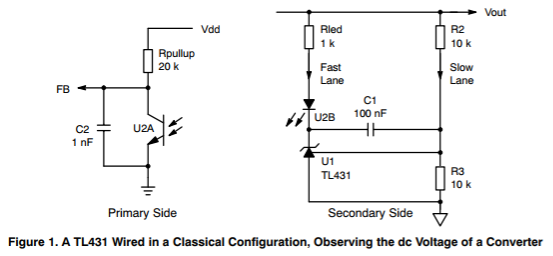
1. C1 in a portion of a switching regulator circuit, from ON Semiconductor’s Application Note AND8327/D — authored in part by the eminent Christoph Basso

   

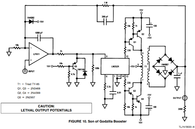
2. The 1000pF cap across the LF411 in the “Son of Godzilla Booster” from National Semiconductor’s AN-272, allegedly written by Jim Williams:

   

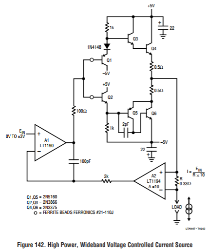
3. The 100pF cap across the LT1190 in a high-power wideband current source, from Linear Technology’s AN47, also by Jim Williams. (In fact there are several other circuits in this appnote that use the same technique.)

   

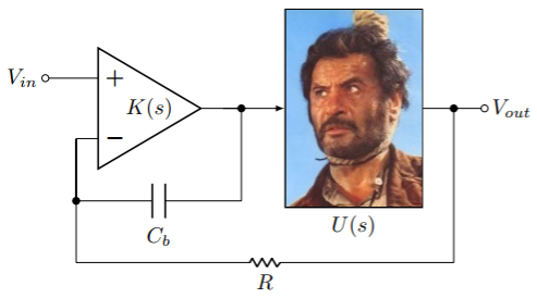
These are examples of circuits with feedback bypass capacitors. In all three cases, we have an error amplifier with gain \( K(s) \), feeding an ugly complex system with some input-to-output gain \( U(s) \) (U for “ugly”) through some equivalent resistance \( R \), along with a capacitor \( C_b \) that bypasses the feedback.

In the AND8327 appnote (“Figure 1” including the TL431), this capacitance is C1 (100nF) and the resistance R is the Thévenin equivalent \( R2 || R3 = 5\text{k}\Omega \); the “ugly” system includes the transconductance of the TL431, the current transfer ratio of the optoisolator, the pullup resistor, and the small-signal equivalent of whatever switching power supply stage relates the input FB to the output Vout.

In the Son of Godzilla Booster, the feedback capacitance is the 1000 pF capacitor across the LF411 and the resistance is the 1M capacitor at the top of the circuit (with 300pF parallel capacitance to provide some high-frequency feedback); the “ugly” system is the LM3524 switching converter, transformer, and rectifier.

In the wideband current source, the feedback capacitance is the 100 pF capacitor across the LT1190, and the resistance is the 2K resistor from the LT1194, which serves to correct any nonlinearities or offsets of the LT1190; the “ugly” system is the LT1194 and the transistor current mirror circuit.

The idea is that \( U(s) \) includes DC and low-frequency feedback that we care about, but for various reasons its high-frequency characteristics can’t be trusted. The capacitor gives us unity-gain feedback at high-frequencies, where feedback from the ugly complex system is attenuated.

Our overall loop gain is \( K(s)F(s) \) where $$F(s) = \dfrac{\frac{U(s)}{R} + C_bs}{\frac{1}{R} + C_bs} = \dfrac{U(s) + RC_bs}{1 + RC_bs}$$ is the net feedback transfer function, derived via Millman’s Theorem. At low frequencies (\( \omega \ll 1/RC_b \)), \( F(s) \approx U(s) \), and at high frequencies \( F(s) \approx 1 + \dfrac{U(s)}{RC_bs} \approx 1. \)

An example

Let’s look at a particular example in more detail. Here let’s say that \( U(s) \) is a unity-gain power amplifier (with some characteristic time constant \( \tau \)) followed by an LC circuit with some parasitic series resistance \( R_s \) in the inductance.

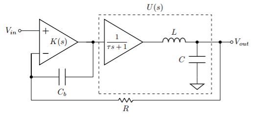
So we can model \( U(s) = \dfrac{1}{\tau s + 1}\cdot\dfrac{1/Cs}{Ls + R_s + 1/Cs} = \dfrac{1}{\tau s + 1}\cdot\dfrac{1}{LCs^2 + R_sCs + 1} \). The LC circuit we can treat as a 2nd-order system, so \( U(s) = \dfrac{1}{\tau s + 1}\cdot\dfrac{1}{s^2/\omega_n{}^2 + 2\zeta s/\omega_n + 1} \) where \( \omega_n = 1/\sqrt{LC} \) and \( \zeta = \frac{R_s}{2}\sqrt{\frac{C}{L}} \). For well-constructed inductors \( \zeta \) will be small: take for example \( L = 100\mu \text{H} \), \( R_s = 0.2 \Omega \), and \( C = 47\mu \text{F} \); this gives us \( \omega \approx 14587 \) rad/s and \( \zeta \approx 0.145 \).

What about the op-amp’s \( K(s) \)? Well, we can approximate \( K(s) = \dfrac{B}{s + B/K_{DC}} \) where \( B \) is the gain-bandwidth product in rad/s, and \( K_{DC} \) is the DC gain. Let’s assume we have a 1MHz GBW opamp with a DC gain of 200,000.

If we choose \( R = 100K\Omega \) and \( C_b = 1\mu F \), we can draw Bode plots of the overall loop gains \( KF \) (with the capacitor \( C_b \)) and \( KU \) (without). Jump past the Python code unless you’re really interested; it’s just there to draw pictures.

import numpy as np
import matplotlib.pyplot as plt

def opamp_tf(B, Kdc):
    def K(s):
        return B/(s+B/Kdc)
    return K

def ugly_tf(L,C,Rs,tau):
    def U(s):
        return 1/(tau*s + 1)/(L*C*s*s + Rs*C*s + 1)
    return U

class LimitFinder():
    def __init__(self):
        self._min = None
        self._max = None
    def __iadd__(self, data):
        newmin = np.min(data)
        newmax = np.max(data)
        if self._min is None:
            self._min = newmin
            self._max = newmax
        else:
            self._min = min(newmin, self._min)
            self._max = max(newmin, self._max)
        return self
    @property
    def min(self):
        return self._min
    @property
    def max(self):
        return self._max
    def ticks(self, delta, clipmin=None, clipmax=None):
        tmin = self.min if clipmin is None else max(clipmin,self.min)
        tmax = self.max if clipmax is None else min(clipmax,self.max)
        return np.arange(tmin//delta*delta,tmax+delta,delta)
    def __repr__(self):
        return "[%s,%s]" % (self.min, self.max)
    
def interpolate_steep(x, ylist, max_interp=100):
    n = len(x)
    ninterp = []
    for y in ylist:
        ymin = np.min(y)
        ymax = np.max(y)
        dyref = np.abs(ymax-ymin)/n
        if dyref < 1e-10:
            alpha = x*0
        else:
            alpha = np.abs(np.diff(y))/dyref
        ninterp.append(alpha)
    ninterp = np.floor(np.max(np.array(ninterp),0))
    ninterp = np.minimum(max_interp, ninterp)
    xinterp = []
    for k in np.argwhere(ninterp > 1):
        x1 = x[k]
        x2 = x[k+1]
        dx = (x2-x1)/ninterp[k]
        xinterp.append(x1+np.arange(1,ninterp[k])*dx)
    return np.hstack(xinterp)
    

def bodeplot(Hfunclist, fig=None, npoints=100, maglimits=None, xlim=None):
    if xlim is None:
        xlim = [-2,6]
    else:
        xlim = np.log10(xlim)
    omega1 = np.logspace(xlim[0],xlim[1],npoints)
    lxlim = [omega1[0],omega1[-1]]
    db = lambda x: 20*np.log10(np.abs(x))
    ang = lambda x: np.angle(x,deg=True)
    ticks = lambda xmin,xmax,delta: np.arange(xmin//delta*delta,xmax+delta,delta)
    if fig is None:
        fig = plt.figure(figsize=(8,6))
    ax1 = fig.add_subplot(2,1,1)
    ax2 = fig.add_subplot(2,1,2)
    omega_additional = interpolate_steep(omega1, [f(Hfunc(1j*omega1)) for f in [db, ang] for Hfunc in Hfunclist], max_interp=200)
    omega = np.union1d(omega1,omega_additional)
    maglim = LimitFinder()
    phaselim = LimitFinder()
    for Hfunc in Hfunclist:
        H = Hfunc(1j*omega)
        ax1.semilogx(omega,db(H))
        maglim += db(H)
        ax2.semilogx(omega,ang(H))
        phaselim += ang(H)
    ax1.set_ylabel(r'$20\, \log_{10} |H(\omega)|$', fontsize=16)
    ylim = [maglim.min, maglim.max]
    if maglimits is None:
        maglimits = (None, None)
    if maglimits[0] is not None:
        ylim[0] = max(maglimits[0], ylim[0])
    if maglimits[1] is not None:
        ylim[1] = min(maglimits[1], ylim[1])
        
    ax1.set_yticks(maglim.ticks(10, clipmin=maglimits[0], clipmax=maglimits[1]))
    ax1.set_ylim(1.05*ylim[0]-0.05*ylim[1],1.05*ylim[1]-0.05*ylim[0])
    ax1.grid('on')
    
    ax2.set_yticks(phaselim.ticks(15))
    if phaselim.min < -175 and phaselim.max > 175:
        ax2.set_ylim(-180,180)
    ax2.set_ylabel(r'$\measuredangle H(\omega)$',fontsize=16)
    ax2.set_xlabel(r'$\omega$ (rad/s)',fontsize=16)
    ax2.grid('on')
    return (fig,ax1,ax2)

Kdc = 2e5
B = 2*np.pi*1e6
tau_opamp = Kdc/B
K = opamp_tf(B=B, Kdc=Kdc)
Utau = 500e-6
L = 100e-6
Rs = 0.2
C = 47e-6
U = ugly_tf(L=L, Rs=Rs, C=C, tau=Utau)
R = 100e3
Cb = 1e-6
tau_fb = R*Cb
F = lambda s: (U(s)+R*Cb*s)/(1+R*Cb*s)
loop1 = lambda s: K(s)*U(s)
loop2 = lambda s: K(s)*F(s)
fig = plt.figure(figsize=(10,10))
_, ax1, ax2 = bodeplot([loop1, loop2], fig=fig, maglimits=[0,None])
for ax in [ax1,ax2]:
    ax.legend(['K*U','K*F'])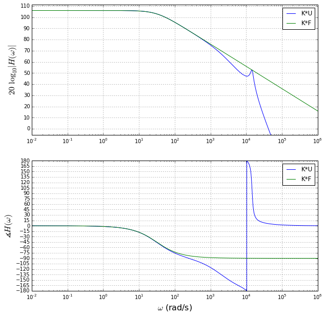

There’s a big difference between the loop gain with the feedback bypass capacitor (KF) and the loop gain without it (KU). Without the feedback bypass capacitor, we have a really ugly transfer function with more than 180 degree phase lag long before it gets to unity gain (and nearly 360 degree phase lag at unity gain). With the feedback bypass capacitor, we can achieve essentially a first-order transfer function for open-loop gain.

Just because the open-loop gain is well behaved, it doesn’t mean the closed-loop transfer function is very smooth, but it does ensure stability. Let’s draw a Bode plot of the closed-loop transfer function. We’ll also use the scipy.signal.lti objects to show step responses (although there’s some algebra to get this).

# closed-loop transfer functions
cloop1 = lambda s: K(s)*U(s)/(1+K(s)*F(s))
Uden   = lambda s: 1/U(s)
cloop2 = lambda s: Kdc*(1+tau_fb*s)/(Uden(s)*(tau_opamp*s+1)*(tau_fb*s+1) + Kdc*(1 + tau_fb*s*Uden(s)))
cloopdiff = lambda s: cloop1(s)-cloop2(s)

def maxdiff(f1,f2,x):
    return np.max(np.abs(f1(x) - f2(x)))

# are these the same transfer function? (check my algebra)
stest = 1j*np.logspace(-6,6,1000)
print "cloop1-cloop2:", maxdiff(cloop1, cloop2, stest)

import scipy.signal
from numpy.polynomial.polynomial import Polynomial
P1 = Polynomial(1)

# 1/(tau*s + 1)/(L*C*s*s + Rs*C*s + 1)
pUden = P1 * [1,Utau] * [1,Rs*C,L*C]

# scipy.signal.lti expects *descending* order
def make_closedTF(tau):
    tau_s        = 0 if tau is None else Polynomial([0,tau])
    return scipy.signal.lti(# Numerator
                            (P1 * Kdc * (tau_s + 1)).coef[::-1],
                            # Denominator
                            ( (pUden * [1,tau_opamp] * (tau_s + 1))
                             + Kdc * (1 + pUden*tau_s)
                            ).coef[::-1]
                            )
closedTF = make_closedTF(tau_fb)

closedTF_H = lambda s: closedTF.freqresp(s/1j)[1]

print "cloop1-LTI", maxdiff(cloop1, closedTF_H, stest)

cloop1-cloop2: 6.66200242854e-16
cloop1-LTI 1.26858466865e-15

fig = plt.figure(figsize=(10,10))
bodeplot([cloop1, cloop2, closedTF_H], fig=fig, maglimits=[-60,None])

(<matplotlib.figure.Figure at 0x14f1d7050>,
 <matplotlib.axes._subplots.AxesSubplot at 0x14f1d7910>,
 <matplotlib.axes._subplots.AxesSubplot at 0x140dc0c50>)

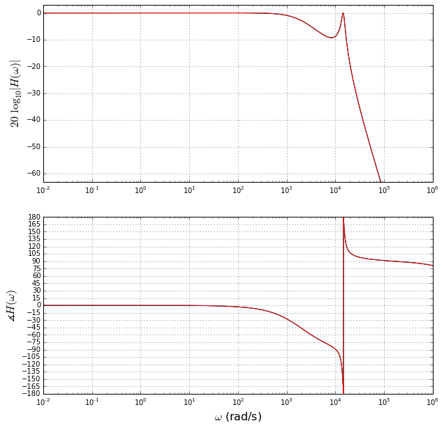
This closed-loop transfer function is mostly well-behaved, although it does have a resonance due to the LC circuit. Here are step responses for various values of \( \tau = RC_b \):

fig=plt.figure(figsize=(10,8))
ax=fig.add_subplot(1,1,1)
taulist = tau_fb * np.array([0.0005, 0.001, 0.01, 0.1, 1.0])
colors = 'gykbr'
for k,tauval in enumerate(taulist):
    closedTF = make_closedTF(tauval)
    t,x=closedTF.step(T=np.arange(0,0.01,0.00001))
    ax.plot(t,x, color=colors[k])
ax.legend(['%g us' % (tau*1e6) for tau in taulist])
ax.grid('on')
ax.set_xlabel('t')
ax.set_ylabel('y')

<matplotlib.text.Text at 0x146b3d6d0>

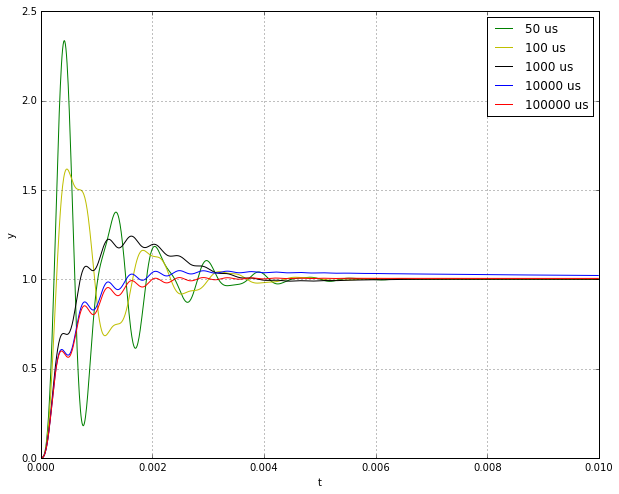
Essentially we have a tradeoff; by increasing the time constant (larger feedback bypass capacitance) we get slower response, but more stable. The circuit exhibits a step response with ringing with small feedback capacitance, and is unstable with no feedback capacitance.

Other examples

This technique is very powerful; I’ve used it several times in my career. One memorable occasion was a battery charger using a 95V Vicor FlatPAC switching power converter. (Designs I created using the Vicor converters both predated and followed the notorious William Tango Foxtrot design I wrote about a couple of years ago.) The FlatPAC converters have a trim circuit that allows trimming between 50% and 110% of nominal output voltage:

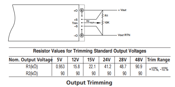
Unfortunately the trim circuit was originally intended to be a manual, potentiometer-based voltage adjustment. Vicor now has an application note on using it as a constant-current battery charger; at the time I created my design, they had some appnote about constant-current use, but I don’t think it went into as much detail, and I had to figure out the hard way that the trim pin had a nonlinear, bandwidth-limited response that was not well-documented, so I used an op-amp to control the trim pin, and in went the feedback bypass capacitor to save the day.

Op-amps have these feedback capacitors, too!

You won’t just find this used in application circuits. In fact, almost all op-amps have an internal feedback bypass capacitor for frequency compensation; here’s the design of the ubiquitous (and awful! please use a better one!) 741 op-amp:

(Image from Wikipedia)

The 30pF capacitor is an internal feedback capacitor that reduces the high-frequency gain of the op-amp, in order to allow the amplifier to have a predictable transfer function that is stable at unity-gain.

Isn’t it just an integrator?

Another way of thinking about the RC stabilizing technique is that it forms an integrator:

If you go through the circuit analysis, you can derive that the gain from \( V_{out} \) to the output of the op-amp is $$G(s) = \frac{-K}{1 + (1+K)RC_b s}$$

If the op-amp gain K is large, then \( G(s) \approx -1/RC_b s \) and we have an ideal integrator… but the op-amp’s low-frequency gain isn’t infinite. A Bode plot of the integrator’s transfer function (with the sign reversed) versus the op-amp’s open-loop gain shows that we’re basically just creating a “virtual” op-amp with much lower gain-bandwidth product:

fig = plt.figure(figsize=(10,10))

K = opamp_tf(B=B, Kdc=Kdc)
integ = lambda s: K(s)/(1 + R*Cb*s + K(s)*R*Cb*s)
_, ax1, ax2 = bodeplot([H1, integ], fig=fig, maglimits=[-60,None], xlim=[1e-6,1e6])
for ax in [ax1,ax2]:
    ax.legend(['K (opamp)','RC integrator'])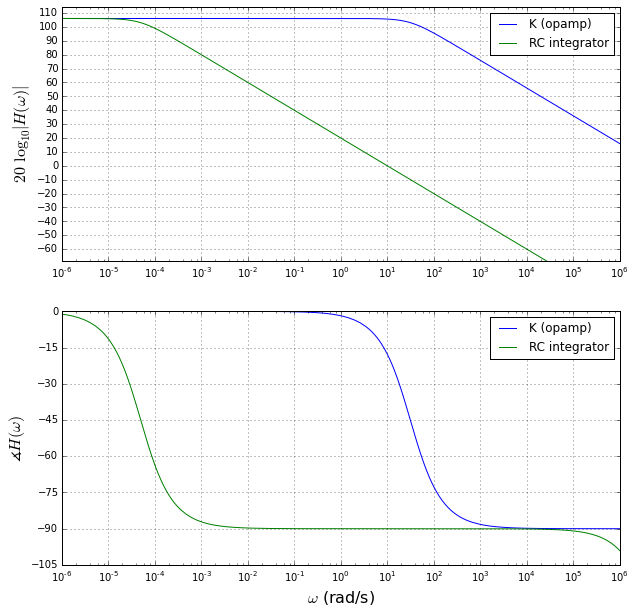

The analysis above isn’t completely correct, however; it shows the feedback loop transfer function, but neglects the transfer function from the \( + \) terminal of the op-amp to its output, which we can add:

$$ V_{opamp,out} = \frac{-KV_{out} + K(1 + RC_b s)V_{in}}{1 + (1+K)RC_b s} $$

This has an additional zero for the transfer function from \( V_{in} \) to op-amp output, which essentially creates a gain of 1 between the cutoff frequency \( \omega_c = 1/RC_b \) and the op-amp’s gain-bandwidth.

Wrap-up

Feedback bypass capacitors are really useful! They let you use an op-amp to take low-frequency feedback from some ugly, nonlinear, slow system, but stabilize the control loop by taking high-frequency feedback from the op-amp output itself, forming a unity gain at high frequencies. I recommend putting this in your bag of circuit-design tricks.

On a related subject: Jim Williams has a nice writeup called “The Oscillation Problem (Frequency Compensation without Tears)” in Linear Technology’s AN18 that gives some good practical advice without getting into any control theory.)

Happy New Year!

P.S. I need to point out another entry to the Hall of Shame. While doing some additional research for this article, I looked up National Semiconductor’s Application Note 4: Monolithic Op Amp — The Universal Linear Component, written by legendary chip designer Bob Widlar and published in April 1968. National was acquired by Texas Instruments in 2011, and you can still find AN4, but it’s been “revised” as TI’s SNOA650B. (I managed to find an earlier version of the National PDF on a webpage at Colorado State University.) The “revised” version omits any mention of Widlar as author of the appnote, and the documentation dwarves at TI have assiduously replaced “National Semiconductor” with “Texas Instruments”… but haven’t bothered to “revise” any other aspects of the appnote, including the fact that the abstract says

The cost of monolithic amplifiers is now less than \$2.00, in large quantities, which makes it attractive to design them into circuits where they would not otherwise be considered.

and later on

Although the designs presented use the LM101 operational amplifier and the LM102 voltage follower produced by Texas Instruments

Hello… it’s 2017, not 1968; I can buy an LM358 op-amp for less than 10 cents in 1K quantities, and there are no more LM102 voltage followers; they were long gone before TI ever got their hands on National. Someone bothered to change that sentence to say “Texas Instruments” rather than “National Semiconductor” but didn’t bother to check it for factual correctness.

I like many of TI’s chips, and am amazed at what kind of clever products come out of their factory, but I really wish they would have just published the old National appnotes in their original form, as historical — but still invaluable — documents. The national.com website is gone, and sorely missed. It makes me wish I had kept some of those databooks-on-CD-ROM that the semiconductor manufacturers put out in the late 1990’s, in those few years between the era of paperweight databooks and the era of ephemeral publications on the Internet.

I hope TI will correct this injustice.

© 2017 Jason M. Sachs, all rights reserved.

Sign in