Linear Regression with Evenly-Spaced Abscissae

What a boring title. I wish I could come up with something snazzier. One word I learned today is studentization, which is just the normalization of errors in a curve-fitting exercise by the sample standard deviation (e.g. point \( x_i \) is \( 0.3\hat{\sigma} \) from the best-fit linear curve, so \( \frac{x_i - \hat{x}_i}{\hat{\sigma}} = 0.3 \)) — Studentize me! would have been nice, but I couldn’t work it into the topic for today. Oh well.

I needed a little break from our tour of linear feedback shift registers — and maybe you do too — so I thought I’d share a little insight in curve-fitting I ran across about ten years ago. What we’re going to do today is do a bunch of linear algebra, so that we can handle all the yucky math ahead of time, and then compute something useful and simple without having to touch the linear algebra again.

Let’s look at a linear regression problem. Ugh. Statisticians need to band together and come up with some more exciting terms. All this means is to fit a line to some data.

import numpy as np
import matplotlib.pyplot as plt
%matplotlib inline

np.random.seed(123)
t = np.arange(0,1,0.05)
n = np.random.randn(*t.shape)*0.02
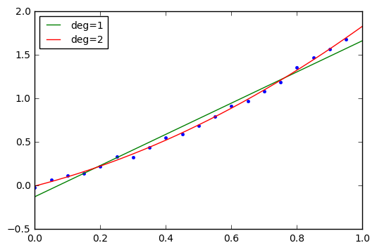
y = 0.8*t*t + t + n
plt.plot(t,y,'.')

# Fit a line and a parabola, and plot them
t_theo = np.linspace(0, 1, 1000)
for deg in [1,2]:
    p = np.polyfit(t,y,deg)
    print "Degree %d: p=%s" % (deg,p)
    plt.plot(t_theo, np.polyval(p,t_theo),label='deg=%d'%deg)
plt.legend(loc='best', fontsize=10);

Degree 1: p=[ 1.79183292 -0.12683228]
Degree 2: p=[ 0.86334813  0.9716522  -0.00380517]

The numpy.polyfit function is the easy thing to use when fitting any polynomial (linear or not). It uses a least-squares fit, something explored by Carl Friedrich Gauss, and since today is Gauss’s birthday, it seems like a fitting tribute. (Pun intended.)

Here comes the math:

We call numpy.polyfit on a bunch of data \( (x_i, y_i) \) and we get a vector of coefficients \( p_k \) such that the sum of the squared errors \( E \) is minimized:

$$E = \sum\limits_i (\hat{y}_i - y_i)^2$$

with the estimated value \( \hat{y}_i \) defined as the evaluation of the polynomial at each point:

$$\hat{y}_i = p(x_i) = p_0 + p_1x_i + p_2x_i{}^2 + \ldots + p_nx_i{}^n$$

(Note: polyfit returns the coefficients from most-significant to least-significant, e.g. it gives you a vector \( \begin{bmatrix}p_n & p_{n-1} & \ldots & p_2 & p_1 & p_0\end{bmatrix} \). Just make sure you’re aware of this order.)

Okay, here I am talking about least-squares, but a few years back I wrote an article on Chebyshev approximation, which is slightly different. Here’s the thing to note:

• When you are approximating a function and trying to fit a polynomial to it, so that you can choose the x-coordinates (abscissae) of the data, and the error is approximation error rather than noise, then Chebyshev approximation is the thing to use.
• When you are trying to fit a polynomial to noisy data that you’re just stuck with — well, think twice; I would not recommend more than cubic — then least-squares is the best approach.
• If you have noisy data from an experiment where you have the freedom to choose the x-coordinates — for example, if you are trying to understand the relationship for a sensor between the physical quantity it is sensing, and its output signal — then it’s kind of a gray area whether to use evenly-spaced points or Chebyshev nodes. As the number of samples goes up, the difference between the approaches goes down, and for 10 or more samples, I would just as well choose evenly-spaced data for its neatness.

Basically, Chebyshev approximation exploits some of the smoothness properties of ordinary functions to come up with a result that approximately minimizes the maximum error over an interval. With least-squares approximation, we don’t care about the maximum error so much as the sum of the squares of the error. If you’ve read this and are scratching your head, just forget I mentioned the Chebyshev stuff, and move on.

What does polyfit do? Well, under the hood it uses least squares to fit a linear sum of basis functions, where the basis functions are \( 1, x, x^2, \ldots, x^n \).

This is the essence of least-squares analysis: given samples \( (x_i, y_i) \), along with some choice of basis functions \( a_0(x), a_1(x), a_2(x), \ldots a_{n-1}(x) \) — watch out, here there are \( n \) terms whereas with \( n \)th degree polynomials there are \( n+1 \) terms — then, through the magic of linear algebra, we can find coefficients \( c_0, c_1, c_2, \ldots c_{n-1} \) such that the best fit function \( \hat{f}(x) = \sum\limits_{j=0}^{n-1} c_ja_j(x) \) minimizes the total squared error \( E = \sum\limits_i (y_i - \hat{f}(x_i))^2 \).

Essentially \( E \) is a “score” that we try to minimize over the entire sample set. The resulting function \( \hat{f}(x) \) usually isn’t going to pass through any of the points, but it stays nearby enough to keep \( E \) as low as possible.

The math to do this is fairly straightforward. You form the following matrix:

$$\mathbf{A} = \begin{bmatrix} a_0(x_0) & a_1(x_0) & a_2(x_0) & \ldots & a_{n-1}(x_0) \cr a_0(x_1) & a_1(x_1) & a_2(x_1) & \ldots & a_{n-1}(x_1) \cr a_0(x_2) & a_1(x_2) & a_2(x_2) & \ldots & a_{n-1}(x_2) \cr \vdots & \vdots & \vdots & & \vdots \cr a_0(x_{m-1}) & a_1(x_{m-1}) & a_2(x_{m-1}) & \ldots & a_{n-1}(x_{m-1}) \cr \end{bmatrix}$$

so that each column represents one basis function evaluated at all the sample points, and each row represents one sample point evaluated using all of the functions, and then we have the matrix equation

$$\mathbf{r} = \mathbf{y} - \mathbf{A}\mathbf{c} $$

where

$$\mathbf{y} = \begin{bmatrix} y_0 \cr y_1 \cr y_2 \cr \vdots \cr y_{m-1} \end{bmatrix}, \qquad \mathbf{c} = \begin{bmatrix} c_0 \cr c_1 \cr c_2 \cr \vdots \cr c_{n-1} \end{bmatrix}$$

It turns out that this has the least-squares solution (which minimizes the vector norm of the residual \( \|\mathbf{r}\|^2 \)) of

$$\mathbf{A}^T\mathbf{A}\mathbf{c} = \mathbf{A}^T\mathbf{y}$$

or

$$\mathbf{c} = (\mathbf{A}^T\mathbf{A})^{-1}\mathbf{A}^T\mathbf{y}.$$

Anyway, the numpy.linalg.lstsq function will do all that for you. You just need to form the \( \mathbf{A} \) matrix yourself. The numpy.polyfit function will do that part for you, too.

If we wanted to use numpy.linalg.lstsq instead of numpy.polyfit for the curve-fitting exercise, we could do it ourselves:

# Fit a line and a parabola, and plot them
plt.plot(t,y,'.')

t_theo = np.linspace(0, 1, 1000)
for deg in [1,2]:
    # First form the A matrix.
    # Put basis functions in rows and then transpose.
    A = np.vstack([t**j for j in xrange(deg+1)]).T
    # Then call lstsq(), and throw away everything but the coefficients
    p, _, _, _ = np.linalg.lstsq(A,y)
    print "Degree %d: p=%s" % (deg,p)
    y_theo = sum(pj*(t_theo**j) for j,pj in enumerate(p))
    plt.plot(t_theo, y_theo, label='deg=%d'%deg)
plt.legend(loc='best', fontsize=10);

Degree 1: p=[-0.12683228  1.79183292]
Degree 2: p=[-0.00380517  0.9716522   0.86334813]

There. Same result, we just have the polynomial coefficients in ascending rather than descending order.

Let’s look at the \( \mathbf{A} \) matrix for the quadratic case, and you can see fairly easily that the columns are just the basis functions \( 1 \), \( x \), and \( x^2 \):

A

array([[ 1.    ,  0.    ,  0.    ],
       [ 1.    ,  0.05  ,  0.0025],
       [ 1.    ,  0.1   ,  0.01  ],
       [ 1.    ,  0.15  ,  0.0225],
       [ 1.    ,  0.2   ,  0.04  ],
       [ 1.    ,  0.25  ,  0.0625],
       [ 1.    ,  0.3   ,  0.09  ],
       [ 1.    ,  0.35  ,  0.1225],
       [ 1.    ,  0.4   ,  0.16  ],
       [ 1.    ,  0.45  ,  0.2025],
       [ 1.    ,  0.5   ,  0.25  ],
       [ 1.    ,  0.55  ,  0.3025],
       [ 1.    ,  0.6   ,  0.36  ],
       [ 1.    ,  0.65  ,  0.4225],
       [ 1.    ,  0.7   ,  0.49  ],
       [ 1.    ,  0.75  ,  0.5625],
       [ 1.    ,  0.8   ,  0.64  ],
       [ 1.    ,  0.85  ,  0.7225],
       [ 1.    ,  0.9   ,  0.81  ],
       [ 1.    ,  0.95  ,  0.9025]])

I used this technique in LFSR Part XIII with a constant and an exponential function.

Now, here comes the interesting part.

Exploitation of Linearity

Let’s go back to the least-squares solution:

$$\mathbf{c} = (\mathbf{A}^T\mathbf{A})^{-1}\mathbf{A}^T\mathbf{y}$$

which we can write as

$$\mathbf{c} = \mathbf{\Gamma}\mathbf{y}$$

where \( \mathbf{\Gamma} = (\mathbf{A}^T\mathbf{A})^{-1}\mathbf{A}^T \) is all that yucky matrix junk that depends only on the basis functions and on the x-coordinate values. The matrix \( \mathbf{\Gamma} \) is not dependent on the y-coordinate values.

And if we have evenly-spaced x-coordinate values \( x_i = i\Delta x+x_0 \), something special happens. Let’s choose basis functions \( a_0(x) = 1 \) and \( a_1(x_i) = (x_i - x_0)/\Delta x - \bar{i} = i - \bar{i} \) with \( \bar{i} = \frac{m-1}{2} \):

for m in xrange(2, 10):
    a0 = np.ones(m)
    a1 = np.arange(m, dtype=np.float64) - (m-1)/2.0
    A = np.vstack([a0,a1]).T
    print "m=%d, A=\n%s" % (m, A)
    gamma = np.dot(
                np.linalg.inv(np.dot(A.T, A)),
                A.T)
    q = gamma[1,1] - gamma[1,0]
    print "gamma.T=\n%s" % gamma.T
    print "q=%f\n-------" % q

m=2, A=
[[ 1.  -0.5]
 [ 1.   0.5]]
gamma.T=
[[ 0.5 -1. ]
 [ 0.5  1. ]]
q=2.000000
-------
m=3, A=
[[ 1. -1.]
 [ 1.  0.]
 [ 1.  1.]]
gamma.T=
[[ 0.33333333 -0.5       ]
 [ 0.33333333  0.        ]
 [ 0.33333333  0.5       ]]
q=0.500000
-------
m=4, A=
[[ 1.  -1.5]
 [ 1.  -0.5]
 [ 1.   0.5]
 [ 1.   1.5]]
gamma.T=
[[ 0.25 -0.3 ]
 [ 0.25 -0.1 ]
 [ 0.25  0.1 ]
 [ 0.25  0.3 ]]
q=0.200000
-------
m=5, A=
[[ 1. -2.]
 [ 1. -1.]
 [ 1.  0.]
 [ 1.  1.]
 [ 1.  2.]]
gamma.T=
[[ 0.2 -0.2]
 [ 0.2 -0.1]
 [ 0.2  0. ]
 [ 0.2  0.1]
 [ 0.2  0.2]]
q=0.100000
-------
m=6, A=
[[ 1.  -2.5]
 [ 1.  -1.5]
 [ 1.  -0.5]
 [ 1.   0.5]
 [ 1.   1.5]
 [ 1.   2.5]]
gamma.T=
[[ 0.16666667 -0.14285714]
 [ 0.16666667 -0.08571429]
 [ 0.16666667 -0.02857143]
 [ 0.16666667  0.02857143]
 [ 0.16666667  0.08571429]
 [ 0.16666667  0.14285714]]
q=0.057143
-------
m=7, A=
[[ 1. -3.]
 [ 1. -2.]
 [ 1. -1.]
 [ 1.  0.]
 [ 1.  1.]
 [ 1.  2.]
 [ 1.  3.]]
gamma.T=
[[ 0.14285714 -0.10714286]
 [ 0.14285714 -0.07142857]
 [ 0.14285714 -0.03571429]
 [ 0.14285714  0.        ]
 [ 0.14285714  0.03571429]
 [ 0.14285714  0.07142857]
 [ 0.14285714  0.10714286]]
q=0.035714
-------
m=8, A=
[[ 1.  -3.5]
 [ 1.  -2.5]
 [ 1.  -1.5]
 [ 1.  -0.5]
 [ 1.   0.5]
 [ 1.   1.5]
 [ 1.   2.5]
 [ 1.   3.5]]
gamma.T=
[[ 0.125      -0.08333333]
 [ 0.125      -0.05952381]
 [ 0.125      -0.03571429]
 [ 0.125      -0.01190476]
 [ 0.125       0.01190476]
 [ 0.125       0.03571429]
 [ 0.125       0.05952381]
 [ 0.125       0.08333333]]
q=0.023810
-------
m=9, A=
[[ 1. -4.]
 [ 1. -3.]
 [ 1. -2.]
 [ 1. -1.]
 [ 1.  0.]
 [ 1.  1.]
 [ 1.  2.]
 [ 1.  3.]
 [ 1.  4.]]
gamma.T=
[[ 0.11111111 -0.06666667]
 [ 0.11111111 -0.05      ]
 [ 0.11111111 -0.03333333]
 [ 0.11111111 -0.01666667]
 [ 0.11111111  0.        ]
 [ 0.11111111  0.01666667]
 [ 0.11111111  0.03333333]
 [ 0.11111111  0.05      ]
 [ 0.11111111  0.06666667]]
q=0.016667
-------

It turns out that \( \mathbf{\Gamma} \) has a very special form. The coefficients of its first row \( \mathbf{\Gamma}_0 \) are all identical and are equal to \( \frac{1}{m} \). The coefficients of its second row \( \mathbf{\Gamma}_1 \) are a linear series \( (i-\bar{i})\cdot q \) with \( \bar{i} = \frac{m-1}{2} \) and \( q=\frac{12}{m^3 - m} \).

So What?

Time to play that Miles Davis again.

OK, for a linear fit we have

$$\mathbf{c} = \begin{bmatrix}c_0 \cr c_1\end{bmatrix} = \begin{bmatrix}\mathbf{\Gamma}_0 \cr \mathbf{\Gamma}_1\end{bmatrix} \mathbf{y}$$

The value \( c_0 \) is just the mean value of the \( y \) values. That’s easy.

The value \( c_1 \) is a weighted sum of \( y \) values, with weights that form an arithmetic progression.

For \( m=5 \), for instance, \( q=\frac{12}{120} = \frac{1}{10} \) and we get \( c_1 = \frac{1}{10}(-2y_0 -1y_1 +0y_2 + y_3 + 2y_4) \). (Odd values of \( m \) have a zero term in the middle.)

For \( m=6 \), we have \( q=\frac{12}{210} = \frac{2}{35} \) and we get \( c_1 = \frac{2}{35}(-\frac{5}{2}y_0 -\frac{3}{2}y_1 -\frac{1}{2}y_2 + \frac{3}{2}y_3 + \frac{5}{2}y_4) \).

Then the best fit line has the equation \( y = c_0 + c_1(i-\bar{i}) = c_0 + \frac{c_1}{\Delta x}(x_i - x_0) - c_1\bar{i} \).

This is all yucky algebra, and kind of hard to wrap your head around it, so let’s try it on a sample data set to see how it works in practice.

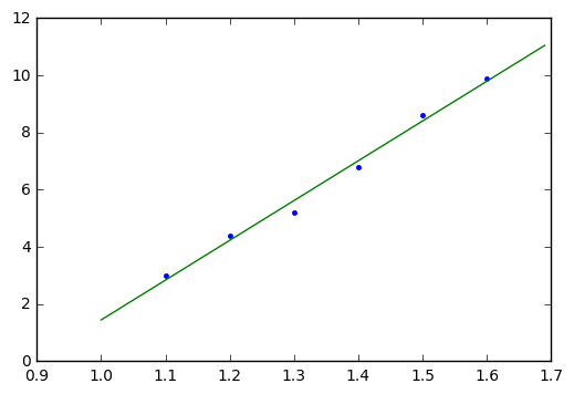
x = np.array([1.1, 1.2, 1.3, 1.4, 1.5, 1.6])
y = np.array([3.0, 4.4, 5.2, 6.8, 8.6, 9.9])

Now here we have \( m=6 \) and \( x_i = 1.1 + 0.1\cdot i = x_0 + i\Delta x \) so \( x_0 = 1.1 \) and \( \Delta x = 0.1 \).

We’re going to calculate \( c_0 \) and \( c_1 \) more explicitly here:

m = 6
q = 12.0/(m**3 - m)
c0 = np.mean(y)
c1 = q*(-2.5*y[0] - 1.5*y[1] - 0.5*y[2] + 0.5*y[3] + 1.5*y[4] + 2.5*y[5])
x0 = 1.1
dx = 0.1
c0, c1

(6.3166666666666664, 1.391428571428571)

line_m = c1/dx
ibar = (m-1)/2.0
line_b = c0 - line_m*x0 - c1*ibar
line_m, line_b

(13.914285714285709, -12.467619047619042)

plt.plot(x,y,'.')
x_theo = np.arange(1,1.7,0.01)
plt.plot(x_theo, line_m*x_theo + line_b);

We can do the same thing in general, not just for a specific data set. What this means is that we can write code to calculate the best-fit line slope and offset without having to mess around with matrices!

Let’s write a general routine:

def linear_fit_equal_spacing(y, x0, dx):
    """
    Calculates best fit linear coefficients slope, ofs
    such that e = y - (slope*x + ofs) is minimized in a 
    least-squares sense.
    
    The values of x must be equally spaced with x = x0 + i*dx.
    """
    
    m = len(y)
    w = 1.0 / m
    q = 12.0 / (m**3 - m)
    c0 = 0.0
    c1 = 0.0
    ibar = (m-1)/2.0
    for i,y in enumerate(y):
        c0 += y*w
        c1 += y*q*(i-ibar)
    slope = c1/dx
    ofs = c0 - slope*x0 - c1*ibar
    return slope, ofs

slope, ofs = linear_fit_equal_spacing(y, 1.1, 0.1)
print "slope=%f, ofs=%f" % (slope,ofs)
plt.plot(x,y,'.')
x_theo = np.arange(1,1.7,0.01)
plt.plot(x_theo, slope*x_theo + ofs);

slope=13.914286, ofs=-12.467619

Tada!

And that’s my little trick to share for today.

There are more general formulas for estimating linear least squares coefficients, where the x-coordinates are not evenly spaced, and they aren’t much harder to calculate. The common formulas involve sums of the first and second moments of data (\( \sum x, \sum y, \sum x^2, \sum y^2, \sum xy \)).

Wrapup

Linear regression is fitting a linear equation with slope and offset to a series of data points. If we use least-squares fitting, there is a fairly simple set of equations that minimizes the sum of squared errors between the actual data points and the value predicted by the linear equation.

In matrix form, least-squares problems can be expressed as minimizing \( \|\mathbf{r}\|^2 \) where \( \mathbf{r} = \mathbf{y} - \mathbf{A}\mathbf{c} \) for an unknown vector \( \mathbf{c} \). This can be solved as

$$\begin{align}\mathbf{c} &= (\mathbf{A}^T\mathbf{A})^{-1}\mathbf{A}^T\mathbf{y} \cr &= \mathbf{\Gamma}\mathbf{y}\end{align}$$

where \( \mathbf{\Gamma} \) is dependent only on the choice of basis functions that make up \( \mathbf{A} \) and the x-coordinates at which they are taken.

If we wish to use a linear equation, and those x-coordinates are evenly spaced, then the form of \( \mathbf{\Gamma} = \begin{bmatrix}\mathbf{\Gamma}_0 \cr \mathbf{\Gamma}_1\end{bmatrix} \) is very simple, and can be computed easily without needing any linear algebra libraries. \( \mathbf{\Gamma}_0 \) is a uniform vector that produces a mean value calculation, and \( \mathbf{\Gamma}_1 \) is an arithmetic progression that weights the two endpoints most strongly.

© 2018 Jason M. Sachs, all rights reserved.

Sign in