• Audio DSP
• Matlab
• DFT_FFT

1 Introduction

I would like to look at the phase vocoder in a fairly ``abstract'' way today. The purpose of this is to discuss a method for measuring the quality of various phase vocoder algorithms, and building off a proposed measure used in [2]. There will be a bit of time spent in the domain of continuous mathematics, thus defining a phase vocoder function or map rather than an algorithm. We will be using geometric visualizations when possible while pointing out certain group theory similarities for those interested. To start we will make a claim, set forth properties, explore these properties, and amend our original claim based on this exploration. After going through all of this, we should have some new ideas about the phase vocoder and feel sufficiently confident in the given measurement for phase vocoder quality as being a good one.

2 Theory

Let's start by laying out some notation. 

2.1 Notation

    $\alpha = $ time modification factor

    $\beta = $ frequency modification factor

    $x(t) = $ analysis/input time domain signal

    $y(t) = $ synthesis/output time domain signal

    $X(\omega) = $ analysis/input frequency domain signal 

    $Y(\omega) = $ synthesis/output frequency domain signal

When the discussion is more theoretical, we will refer to $x(t)$ as simply $x$, per [1]. We will see why later on. 

2.2 Definitions

The phase vocoder map, $PV(x,\alpha,\beta)$ is defined in the following equation

$$PV\big(x,\alpha,\beta\big) = \int_{-\infty}^{\infty}\big|X\big(\frac{\omega}{\beta},\alpha t\big)\big|\cdot e^{i\phi_{pv}(\omega,t)}d\omega = y(t)$$

where the phase vocoder phase function $\phi_{pv}(t)$ is 

$$\phi_{pv}(\omega, t) = \angle X(\frac{\omega}{\beta},0) + \int_{0}^{t} \frac{d}{dt}\big[\phi(\omega,t)\big] dt = \angle X(\frac{\omega}{\beta},0) + \phi(\omega,t)$$

3 The Weeds

The phase vocoder acts like a map between two sets, the elements of which are signals. These signals have finite energy and can be understood as vectors in a Hilbert Space $\mathbb{H}$, known as a signal space, as elaborated on in [1]. When referring to the vector as a whole, $x(t)$ will be referred to as simply $x$. The domain is the singleton set of the input signal $x(t)$ itself: $\{ x \}$. The co-domain, or range, is the set of all signals $y(t)$ such that $y = PV(x,\alpha,\beta)$ and $\alpha, \beta \in \mathbb{R} - \{0\}$. In total,

$$ PV: \mathcal{X} \mapsto \mathcal{Y}$$

$$ \text{such that } \mathcal{X} = \{(x,\alpha,\beta) | x \in \mathbb{H} \ \text{and } (\alpha,\beta) \in \mathbb{R}^{2} \}  $$

$$\text{and } y \in \mathbb{H} $$

We see here that the input signal $x$ acts like a generator of the co-domain $\mathcal{Y}$. When $\alpha = 1$ and $\beta = 1$, $PV$ acts like the identity map since $PV(x,1,1) = x$. 

Let's look at the characteristics of the input signal which we are modifying (duration and pitch) and see how information in the input signal is related to information in the output. First, let's consider the time characteristics of the signal. Let the duration of $x(t)$ be $N$. Since $x(t)$ is a signal of finite energy, we will assume that $N$ is finite (although this is not necessarily the case). We can pretty easily intuit the effect of time modification $\alpha$: the amplitude envelope of the entire signal is modified such that the relationship of any portion of the amplitude envelope in the original signal is preserved in the output signal. For example, if there is an amplitude swell that lasts a quarter of the length of the input signal, if we want to stretch that signal by a factor of $\alpha = 2$, that same swell would still occupy a quarter of the output signal. Consequently the duration of our output signal is defined as $\frac{N}{\alpha}$. We see the length of the input signal and output signal are linearly related.

Furthermore, consider the frequency characteristics of the output signal. Once again let's start with a geometric visualization: the short term spectrum for any part of the original signal. If at some point in time we observe a frequency $f_{0}$ and its first harmonic $2f_{0}$, then for any frequency modification $\beta$ we still want it to be the case that when $f_{0}$ is mapped to the output $f_{0}^{*}$, that $2f_{0}$ is mapped to $2f_{0}^{*}$. Thus, for a frequency modification factor of $\beta$, we want the frequency domain characteristics of $Y(\omega)$ to be that of $X(\frac{\omega}{\beta})$. Once again the frequency information of the input signal and output signal are linearly related. 

 We have defined the possible values for $\alpha$ and $\beta$ pretty broadly at the outset of this section - all real numbers. Let's think about what that means, look at curious cases, and decide how this defines the type of map the phase vocoder is in the following sections.

3.1 Negative Time Modification Factors

Perhaps what we have said so far seems reasonable for positive modification factors, but the reader might have raised an eyebrow or two when thinking about negative ones. Here let's dig into these negative modification factors and see how it affects our notion of a phase vocoder map.

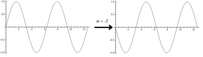
Let's start with time since that is an easier parameter to modify ``negatively''. A time modification factor of $\alpha = -1$ results in the original signal but ``reverse''. In other words all the original time evolution characteristics, such as amplitude envelopes and event timing, are backwards. Furthermore, if we break it down to a Fourier view, this corresponds to conjugation of the o. The latter observation is demonstrated in Figure 1.

3.2 Negative Frequency Modification Factors

When we move to thinking about negative frequency modifications, it may at first seem a bit more difficult to grasp. While the geometric representation we had in the case of negative time modification was enough in the previous section - amplitude envelopes across time - here our geometric representation - amplitude envelopes across frequency - is initially not as robust. Instead, the answer lies in how the Fourier Transform itself operates to generate real signals from complex ones. However, by employing similar tricks we will see that it is well within the realm of what we can understand.

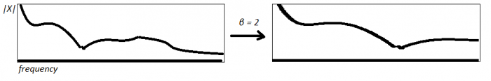
By starting with what we know, let our frequency modification factor be $\beta = 2$. Given the following spectrum on the left, we want to produce the subsequent frequency domain data on the right, as shown in Figure 2. This is again defined in our expression $Y(\omega) = X(\frac{\omega}{\beta})$.

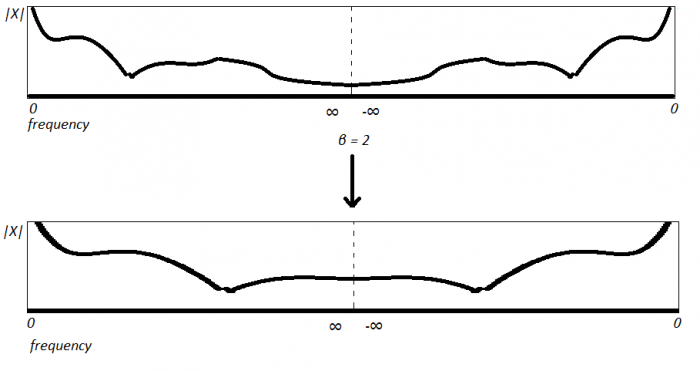
And in fact, another common, and perhaps more useful visualization for our purposes, is shown in Figure 4

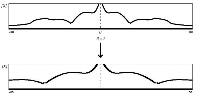
In Figure 4 the notion of negative frequencies is better represented, and perhaps we start to see how this will relate to the topic at hand. Let's start with the simple observation of what negative frequencies even are: complex conjugates of the ``first half'' of the spectrum. For a fourier coefficient $X(\omega) = |X|e^{i\theta}$, its complex conjugate is expressed as $\overline{X(\omega)} = |X|e^{-i\theta}$. Here we will note that if we take a 3D complex view of these frequencies, the conjugates of every positive frequency rotate in the opposite direction of its positive counterpart. This is a consequence of negating the imaginary component. Now let's consider the fourier coefficients which the phase vocoder maps them to given a frequency modification of $\beta > 0$. Let

$$ x(t) = \int_{-\infty}^{\infty}|X(\omega)|e^{-i\theta}d\omega $$

such that  

$$ |X(\omega)| = 0 \ \forall \ \omega \notin \{k,-k\} \ \text{where } |X(k)| = |X(-k)| \neq 0$$

then it follows that

$$ PV(x(t),1,\beta) = y(t)$$

where 

$$|Y(\omega)| = 0 \ \forall \omega \notin \{\beta\cdot k,\beta\cdot-k\} \ \text{such that } |Y(\beta \cdot k)| = |Y(\beta \cdot -k)| = |X(k)|$$

Keeping all this in mind, now consider a frequency modification of $-\beta$. Once again let's take the approach of viewing this modification as having two parts: a positive frequency shift, and then reversing it via the negative part (-1). Using the equation (5), notice the frequencies present in our output signal: 

$$\{- \beta \cdot k,-\beta \cdot -k\} = \{\beta \cdot -k,\beta \cdot k\}$$

These are the same frequencies for a frequency domain modification of $\beta$! This is due to the symmetry of the the spectrum around $\omega = 0$, since we need the negative frequencies to produces a real signal from complex data. Therefore we see that

$$ PV(x(t),\alpha,\beta) = PV(x(t),\alpha,-\beta)$$

3.3 Curious Observation

It might have come across your mind what a frequency or time modification of zero represents in a phase vocoder context. Let's consider this case starting off with time. As we stated earlier, the total time of the input signal and the output are linearly related. So for a time modification factor of $\alpha = 0$, the phase vocoder compresses all of the data in the original signal down to a single point! Interestingly, it seems that $PV(x,0,\beta)$ maps $x$ to an impulse signal. Thus we will say that 

$$PV(x,0,\beta) = \delta_{x}(n)$$

In some sense we see that this is some link to impulse decomposition [3]. However this is more of a tangent than relevant information. 

Furthermore, what does a frequency modification factor of $\beta = 0$ represent? Think back to our geometric conceptualization of frequency modification. We saw that $\beta$ translates the frequency information at a given point to another point in the spectrum. So where is information translated for $\beta = 0$? To frequency `0' or DC! So for $|x| = N$, $PV(x,\alpha, 0)$ generates a singal of length $\alpha N$ that is equal to $DC$ at every point. Thus we will say that 

$$PV(x,\alpha,0) = DC_{x}$$

Finally, if we think about what both of these mean together, we see that $PV(x,0,0)$ gives us a scalar that is equal to the average energy, or DC offset, $DC$, of the input signal $x$. 

3.4 Putting it all together

So what kind of map is the phase vocoder? Or perhaps more importantly: what kind of map do we want the phase vocoder to be? We probably want the PV to be the best kind of map there is: \textit{bijective}! However, given some of the properties we laid out in section 3.2 and 3.3, it seems that our original definition of $(\alpha,\beta) \in \mathbb{R}^{2}$ will not produce a function that is \textit{one-to-one} and \textit{onto}. Let's look at how we can tweak this to result in a map we are happy with. 

We saw in equation (6) that a frequency modification of $\beta$ and $-\beta$ produce an output with the same frequency information. Therefore by defining $\beta \in \mathbb{R}$ the frequency information is not injective, and consequently neither is the PV map as a whole. Furthermore, from section 3.3 we see that for $\beta = 0$, $PV$ is not injective, since multiple input signals $x$ can have the same DC offset. For example, let $x_{1} = sin(t)$ and $x_{2} = cos(t)$. We see that it is the case that 

$$PV(x_{1},\alpha,0) = PV(x_{2},\alpha,0)$$

Moreover, we also see that $PV(x,\alpha,0)$ is the same for all $\alpha$ - as laid out in the beginning of this article. Thus $\beta = 0$ fails a second time in terms of injectivity and therefore must be excluded from the domain. So in order to have bijective frequency information, we must define $\beta \in \mathbb{R}_{> 0}$. 

In terms of time modification, we see that negative values for $\alpha$ actually produce unique output signals. Therefore, unlike is the case for $\beta$, we can include them in the domain for a bijective map. However, once again, as pointed out in 3.3, the result of $PV(x,0,\beta)$ completely destroys the original time information and it cannot be recovered, thus violating injectivity. So if we want to define a bijective phase vocoder map, $\alpha = 0$ must be excluded from the domain. In other words $\alpha \in \mathbb{R} - \{0\}$.

Given these restrictions on $\alpha$ and $\beta$, we see that an output signal of a certain duration and frequency relationship to the input is only possible with a unique $(\alpha_{0},\beta_{0}) \in \mathbb{R}-\{0\} \times \mathbb{R}_{>0}$. Because of this we will say that the phase vocoder map is \textit{one-to-one} and \textit{onto}, in other words a bijection. The reason why defining a bijective phase vocoder map is desirable in the first place is that there must exist an inverse mapping as a consequence of this bijectivity. We will define the inverse phase vocoder map in equation (9).

$$PV^{-1}(x,\alpha,\beta) = PV(y,\frac{1}{\alpha},\frac{1}{\beta})$$

Because $\alpha, \beta \neq 0$, we know that $PV$ is a well-behaved and well-defined mapping. 

In terms of negative time modifications and the inverse PV operation, since there is a $-1$ in both $\alpha$ and $\frac{1}{\alpha}$ in equation (9), when we go from our original signal, to the PV signal, then back to the original signal, there is a phase shift of $\pi$ at each mapping, so a total phase shift of $2\pi$. This gives us the original sinusoid we started off with. Additionally, since we see that the phase information is taken care of, our amplitude envelopes which were initially flipped as a result of the $-1$, are then again flipped in $PV^{-1}$ thus resulting in their original orientation. Again if we take the group theory perspective this acts like a cyclic subgroup $\{ R_{0},R_{180} \}$ of a dihedral group. This last bit seems relevant since dihedral groups are understood in a geometric sense, and here we are conceptualizing the amplitude.

After exploring some of the properties initially set fourth, we have amended our original statement - \textit{that the phase vocoder acts like a map} - to a more powerful and useful conclusion - \textit{this map is bijective}. The fact that the phase vocoder acts like a bijective map is important because it tells us that the signals we are generating from an initial input $x$ are unique for each ordered pair $(\alpha,\beta) \in \mathbb{R} - \{0\} \times \mathbb{R}_{>0}$. Because of this, we can be confident that operations performed on $y \in \mathcal{Y}$ are reflective of the phase vocoder map $PV$ itself, and not some other curious circumstances which were overlooked. \\

In the world of continuous mathematics and analog signals the inverse phase vocoder returns the exact input signal which we originally gave it. However, when working in the world of DSP, certain ``phasey'' artifacts arise in the output phase vocoder signal as a result of spectral leakage and sinusoids of varying frequency. Thus, when we perform the inverse phase vocoder in a digital signal processing context, our signal we get back isn't identical to the one we originally started with. We will see how to use these artifacts to judge the effectiveness of a phase vocoder algorithm.

4 Back to DSP

The properties we just laid out are a bit different when we reenter the digital signal realm. Specifically our frequency modification is no longer injective because of aliasing. They are now cyclic, and for a sampling frequency of $f_{s}$ we redefine 

$$\beta^{*} \equiv \beta \mod f_{s}$$

Furthermore, our choice of $\alpha$ is restricted such that 

$$\alpha \times N \in [1,\infty)$$

since we can't have a signal less than $1$ sample, and we have limited data storage. However, it is near impossible to think of a phase vocoder application that exceeds these bounds, so we will assume these restrictions are met from here on. We will use this notion of the phase vocoder transform as a measure for the resolution of our DSP phase vocoders. 

4.1 Quality Measurement

Laroche and Dolson give us the following Consistency Measure in [2] to quantify the effectiveness of a phase vocoder algorithm. 

$$D_{M} = \frac{\sum_{u = 1}^{P}\sum_{k=0}^{N-1}\big[ | Z(t_{s}^{u},\omega_{k}) | - | X(t_{s}^{u},\omega_{k}) | \big]^{2}}{\sum_{u = 1}^{P}\sum_{k=0}^{N-1} | X(t_{s}^{u},\omega_{k}) |^{2}}$$

This has been slightly modified from the original version: now we are comparing the twice modified signal, $z(t) = PV^{-1}(x(t),\alpha,\beta)$, to the original input, $x(t)$. $D_{M}$ is comparing the squared energy added by the phase vocoder algorithm, to the squared energy of the original signal. If perfect reconstruction is achieved, $D_{M} = 0$. In the following section, we will look at the consistency measure of the Identity Phase Locking algorithm which Laroche and Dolson proposed in [2]. 

4.2 MATLAB Results

The linked MATLAB code performs this forward and inverse phase vocoder operation, and compares the resultant signal with the original one using the consistency measure $D_{M}$. We see these results in Figure 1 and Table 1 where our FFT size is $4096$ with a hop factor of $4$. In light of the aforementioned injectivity failure, $\beta = 1$ in order to avoid aliasing and subsequent distortion. 

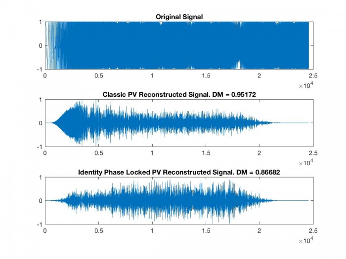
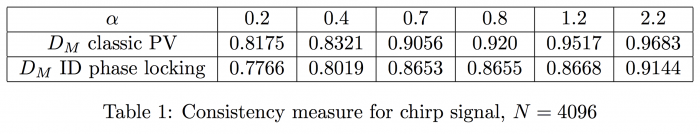
In both phase vocoder reconstructions, we see that a fair amount of energy is added by the phase vocoder. However, we should note that the energy added is exaggerated in our $D_{M}$, since we are performing the discrete phase vocoder algorithm twice, and in the second instance taking in an already phasey signal as input. We see that the Identity Phase Locking algorithm consistently outperforms the classic phase vocoder algorithm in terms of $D_{M}$, as also shown in [2]. 

5 Conclusion

The reader is directed to my phase vocoder master patch for a Max/MSP real-time interactive approach, in order to get a more concrete sense of the PV as a function of three variables. This investigation has brought us through some fringe areas for DSP (Hilbert spaces, group theory, continuous mathematics) in order to give us confidence in using the idea of a phase vocoder transform to judge the quality of a given algorithm. Not only does it give us a slightly different application of the consistency measure $D_{M}$, but we have thought about the phase vocoder and some of the ideas behind it in perhaps a new way: continuously. This is always a healthy practice, as we continue to move through more complete and physical understandings of the powerful ideas employed by digital signal processing. 

References

[1] Robert G. Gallager. Signal Space Concepts. https://pdfs.semanticscholar.org/53f7/0f5b6dc734802cf23624d7912a79f752d102.pdf

[2] Mark Dolson Jean Laroche. Improved Phase Vocoder Time-Scale Modification of

Audio. IEEE, 7(3):323–332, 1999. http://www.cmap.polytechnique.fr/~bacry/MVA/getpapers.php?file=phase_vocoder.pdf&type=pdf

[3]Steven W. Smith. The Scientist and Engineer’s Guide to Digital Signal Processing .California Technical Publishing, San Diego, California, 1997.

Links

MATLAB code

PDF download

my website

Interactive Max/MSP patch

Sign in