Update To: A Wide-Notch Comb Filter

This blog presents alternatives to the wide-notch comb filter described in Reference [1]. That comb filter, which for notational reasons I now call a 2-RRS wide notch comb filter, is shown in Figure 1. I use the "2-RRS" moniker because the comb filter uses two recursive running sum (RRS) networks.

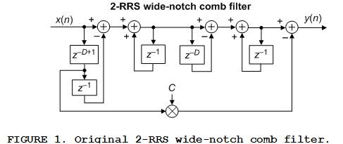
The z-domain transfer function of the 2-RRS wide-notch comb filter, H_2-RRS(z), is:

Encouraged by hirnprinz's Nov. 26th Comment to my Reference [1] blog, I began to experiment with various modifications to the above 2-RRS wide-notch comb filter.

The most noteworthy thing I learned from my experimentation is shown in Figure 2. If we cascade a single recursive running sum (RRS) network to the Figure 1 comb filter, as shown in Figure 2(a), we place frequency magnitude nulls right smack in the middle of the original Figure 1 comb filter's notches. The frequency magnitude response of the Figure 2(a) Enhanced wide-notch comb filter is shown as the solid curve in Figure 2(b).

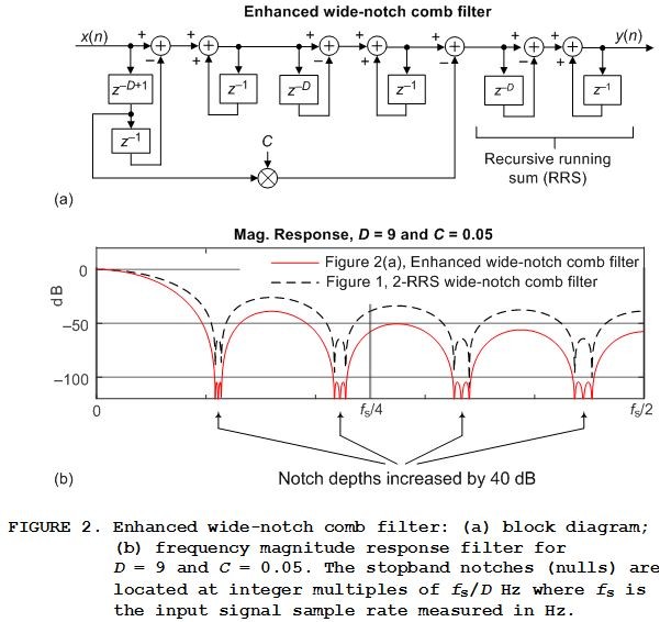
So, at the expense of an additional storage register, a D-length delay line, and two additions per output sample, we have significantly increased the notch attenuation depths.

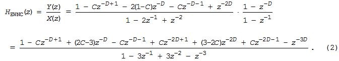
The z-domain transfer function of the Figure 2(a) Enhanced wide-notch comb filter, H_EWNC(z), is the product of H_2-RRS(z) and the transfer function of an RRS network; that is:

This comb filter is linear-phase and its group delay is:

  Enhanced wide-notch comb filter group delay = 3(D-1)/2 samples,

which is always an integer number of samples when D is an odd integer.

In MATLAB code we define the notch width control parameter C and the value of integer D, and use the following to define H_EWNC(z)'s 'B' numerator coefficients and its 'A' denominator coefficients:

  B = [1, zeros(1,D-2), -C, (2*C-3), -C, zeros(1,D-3), C, (3-2*C), C, zeros(1,D-2), -1];

  A = [1, -3, 3, -1];

A Unity-Gain Enhanced Wide-Notch Comb Filter

The DC gain (gain at zero Hz) of the Figure 2(a) Enhanced wide-notch comb filter is:

  H_EWNC DC gain = D³—DC.                                                                   (3)

Appendix B shows how to implement a unity-gain Enhanced wide-notch comb filter.

Other Variations of the 2-RRS Wide-Notch Comb Filter

Fortunately I was able to avoid "Death by Algebra" and successfully investigate other variations of the original 2-RRS wide-notch comb filter.

Those other comb filters, having wider comb notches than the 2-RRS wide-notch comb filter, are described in Appendix A.

Conclusion

I've described four alternatives to the wide-notch comb filter presented in Reference [1]; most notably the deep-notch Enhanced wide-notch comb filter shown in Figure 2(a). (Snippets of MATLAB code were provided.) In addition, Appendix B shows how to implement a unity passband gain version of the Enhanced wide-notch comb filter.

References

[1] R. Lyons, "A Wide-Notch Comb Filter", dsprelated.com Blogs, Nov. 24, 2019, Available online:

https://www.dsprelated.com/showarticle/1308.php

Appendix A: Variations of the Wide-Notch Comb Filter

This appendix describes three additional variations to the Figure 1 original 2-RRS wide-notch comb filter. Here we present the block diagrams, the z-domain transfer functions, and MATLAB code needed to model the three alternative wide-notch comb filters.

3-RRS Wide-Notch Comb Filter

Another comb filter variation I investigated is the linear-phase 3-RRS wide-notch comb filter shown in Figure A-1.

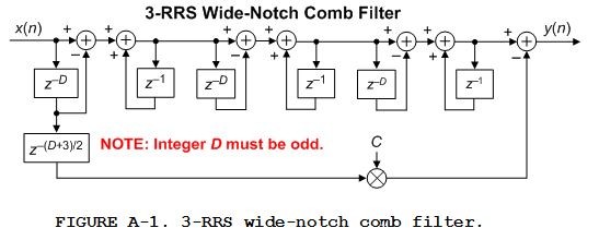
The z-domain transfer functions of the 3-RRS wide-notch comb filter is:

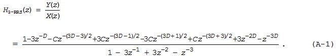
Note that this filter is only stable when D is an odd integer. The group delay of the 3-RRS wide-notch comb filter is:

  3-RRS wide-notch comb filter group delay = 3(D-1)/2 samples.

In MATLAB code we define the notch width control parameter C and the value of integer D, and use the following to define H_3-RRS(z)'s 'B' numerator coefficients and its 'A' denominator coefficients:

  B = [1, zeros(1,D-1), -3, zeros(1,(D-5)/2), -C, 3*C, ...

                                         -3*C, C, zeros(1,(D-5)/2), 3, zeros(1,D-1), -1];

  A = [1, -3, 3, -1];

4-RRS Wide-Notch Comb Filter

The next comb filter variation I explored is the linear-phase 4-RRS wide-notch comb filter shown in Figure A-2.

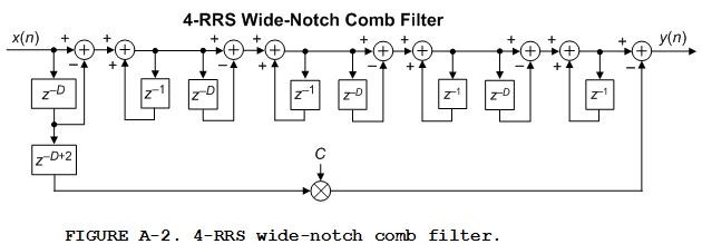
The z-domain transfer functions of the 4-RRS wide-notch comb filter is:

The group delay of the 4-RRS wide-notch comb filter is:

  4-RRS wide-notch comb filter group delay = 2(D-1) samples.

In MATLAB code we define the notch width control parameter C and the value of integer D, and use the following to define H_4-RRS(z)'s 'B' numerator coefficients and its 'A' denominator coefficients:

  B = [1, zeros(1,D-1), -4, zeros(1,D-3), -C, 4*C, 6*(1-C), 4*C, ...

                                       -C, zeros(1,D-3), -4, zeros(1,D-1), 1];

  A = [1, -4, 6, -4, 1];

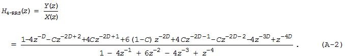
Dual 2-RRS Wide-Notch Comb Filter

The last comb filter variation is the linear-phase Dual 2-RRS wide-notch comb filter formed by cascading a pair of 2-RRS wide-notch comb filters as shown in Figure A-3.

The z-domain transfer function of the Dual 2-RRS wide-notch comb filter is a messy algebraic expression. To model this filter in software we can obtain its rational polynomial transfer function, H_D2-RRS(z), by convolving Eq. (1) with itself as:

The group delay of the Dual wide-notch-notch comb filter is:

  Dual 2-RRS wide-notch comb filter group delay = 2(D-1) samples.

In MATLAB code we define the notch width control parameter C and the value of integer D, and use the following to define H_D2-RRS(z)'s 'B' numerator coefficients and its 'A' denominator coefficients:

  B = [1, zeros(1,D-2), -C, -2*(1-C), -C, zeros(1,D-2), 1];

  A = [1, -2, 1];

  B = conv(B, B);

  A = conv(A, A);

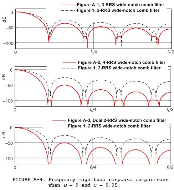
Figure A-4 shows a comparison of the above three comb filters' frequency magnitude responses versus the magnitude response of the original 2-RRS wide-notch comb filter when D = 9 and C = 0.05.

Appendix B: Unity Gain Enhanced Wide-Notch Comb Filter

The simplest method to implement a unity gain (at zero Hz) Enhanced wide-notch comb filter is shown in Figure B-1(a). There we merely scaled the comb filter's output sequence by the reciprocal of the filter's passband gain of D³—DC.

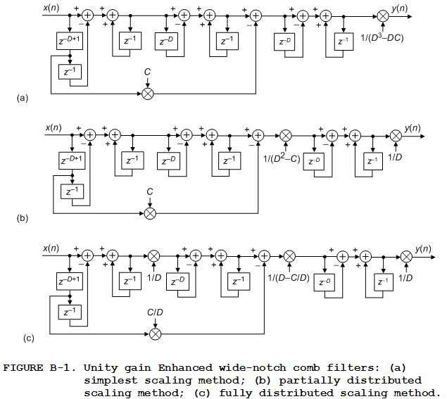
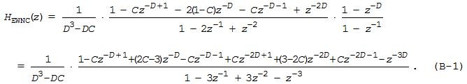
In fixed-point implementations, to reduce the necessary word width of the various accumulators (adders) and two of the z^‑D delay lines, the distributed scaling methods in Figures B-1(b) and B-1(c) can be used. Equation (B-1) gives the transfer function for all the comb filters in Figure B-1:

Sign in