Hello,

I am attempting to plot the result X(f) for various sampling frequencies. I am adjusting the sampling frequencies to intentionally cause aliasing to see the impact on not choosing a frequency at or above the Nyquist rate. 

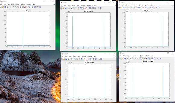
Below are several matlab plots (my f0=10 Hz). The plot labeled CT FT is the continuous time Fourier transform.

As you can see below, it doesn't seem to matter what my sampling frequency is, I get the same results (which I don't think is correct). This makes me think that I am doing something wrong. My guess is that there is some scaling of the x axis (frequency) that I am not properly doing.

 I would expect to see replicas of the CT FT plot at multiples of my Fs. Is this correct?

In this case, why am I not seeing aliasing in any of my plots? 

Thank you for taking time to look at this :)

Here is my matlab code:

f=-40:.001:40;
f0=10;
Xa = 1./(1j*2*pi*(f+f0)); % Note x(t) = u(t) * e^(-j*2*pi*F0*t) where u(t) is the step function
figure(1)
plot(f,abs(Xa))
title('CT FT');


fs=10;
X = 1./(1-exp(-1i*2*pi*(f+f0/fs))); % Note x(t) = u(t) * e^(-j*2*pi*F0*t) where u(t) is the step function
figure(2)
plot(f,abs(X))
title('DTFT, Fs=10');

fs=20;
X = 1./(1-exp(-1i*2*pi*(f+f0/fs)));
figure(3)
plot(f,abs(X))
title('DTFT, Fs=20');

fs=40;
X = 1./(1-exp(-1i*2*pi*(f+f0/fs)));
figure(4)
plot(f,abs(X))
title('DTFT, Fs=40');

fs=100;
X = 1./(1-exp(-1i*2*pi*(f+f0/fs)));
figure(5)
plot(f,abs(X))
title('DTFT, Fs=100');

Do my questions make sense?

With my Matlab code, I've noticed that my plots change a lot if I change the precision of f. f=-10:1:10 produces very different plots then f=-10:.001:10

Does the sampling frequency Fs influence the increment I should use for f when plotting? As in, should I only be progressing my integer numbers?

Thanks.

Hi transient. You cannot compute continuous-time or discrete-time Fourier transforms using a computer. In those transforms the frequency variable is continuous, and we can't implement continuous variables using a computer. Continuous-time and discrete-time Fourier transforms are strictly pencil-and-paper algebra using equations.

What is the theory behind your

   Xa = 1./(1j*2*pi*(f+f0));

command? (I don't recall ever seeing such a command before.)

Hi Rick,

Thank you for your post.
Allow me to elaborate. So I was given the continuous time function below:

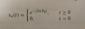
So this (I think) is the same as Xa(t) = e^(-j*2*pi*F0*t) * u(t)

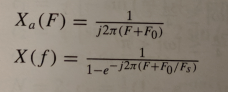
I calculated the continuous time Fourier transform Xa(F) and the Discrete time Fourier transform X(f) as shown below (these match the books answer which is encouraging).

So now, what I would like to do is plot the frequency responses of Xa(F) and X(f). If F0 =10Hz then the plots that I have in my previous post should represent these results. I realize that Fs should be 2*F0 (or more) in order to avoid aliasing. However, no aliasing appears to be present in my plots (even when Fs=F0). Does that make more sense now?

Sorry, I was using matlab short hand this is what this means:

X = 1./(1j*2*pi*(f+f0)); %original line

f is a vector, f0=10, 1j is just the complex value i

so what this line does is that for every value of f (that is f=-40 hz all the way to f = +40Hz with .001 increments) it plugs the value of f into X(f) below. This results in having a new vector X which I use to plot.

X = 1./(1j*2*pi*(f+10));

simpler example:

t = [0 1 2 3];

y = 5.*t;

then, y = [0 5 10 15]

and when I plot(t,y) I am plotting 

x axis points = t = [0 1 2 3]

y axis points = y = [0 5 10 15]

Hi transient. You cannot derive the DTFT equation for your continuous x_a(t) signal. We can only derive the DTFT equations for discrete sequences. I derived the DTFT equation of the sequence:

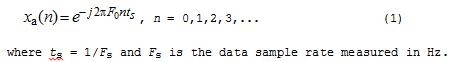
and obtained your X(f) expression:

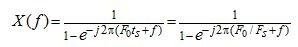
So I now believe your X(f) expression is correct. What we must remember is that the 'f' variable is measured in cycles/sample, and its range is from -0.5 –to- +0.5 (or 0 –to- 1).

Transient, try different values for 'fs' in the following code:

fs = 100;

f = -0.5:.001:0.5;

X = 1./(1-exp(-j*2*pi*(f+f0/fs)));

figure(5)

plot(f,abs(X), '-bs')

title(['DTFT when f_s = ', num2str(fs), ' Hz']);

xlabel('Freq(times f_s)')