Hi all, I'm trying to calculate the AoA and DOA of the received signals according to the Music method. And strangely, the final answer gives me the result in the figure below. According to the share code I had difficulties calculating the "SP(iangl)" due to matrix mismatches, hence I adapted my code as below. I wanted to reproduce the same thing as in the article "SUPER-RESOLUTION ULTRAWIDEBAND ULTRASOUND IMAGING USINGFOCUSED FREQUENCY TIME REVERSAL MUSIC" which shows the angle peaks of two persons arriving, on the spectrogram. Unfortunately, the answer I get gives me two double lines located at the angle between [-90:-80] degrees. The minimum distance between the two persons and the smartphone is 80cm. Is the result below correct? I'm having trouble calculating the DoA correctly and ask for help from the Matlab code below and suggestions. Here is my code and figures:

function [] =  Bartlett_algorithm_dao(signal)
degree_inradian = pi/180;
radian_degree = 180/pi;
twp = 2*pi;
d = 5
wave =2; %number of DOA
theta = [-60 -30 30 60];
SNR = 20;
n = 512;
A = exp(-j*twp*d.'*cos(theta*degree_inradian))'%directio matrix
signal_data = signal;%      generated signal
X = A.*signal_data
X1 = awgn(X, SNR);
Rxx =X1*X1'/n
[EV,D] = eig(Rxx)
EVA = diag(D)'
[EVA,I] = sort(EVA)
EVA = fliplr(EVA)
EV = fliplr(EV(:,I))
%Music method
for iangl = 1:361
angle(iangl) = (iangl-180)/2
phim = degree_inradian*angle(iangl)
a = exp(-j*twp*d*cos(phim)).'
L = wave
En = EV(:,L+1:3)
SP= (En*a').*(a*En')./En.^2
SP(iangl,:) = abs((1./1-(SP(1,:))))
end
%Plot figure
SP = abs(SP)
SPmax = max(SP(iangl))
SP = 10*log10(SP/SPmax)
h = plot(angle, SP)
set(h,'Linewidth', 4)
xlabel('angle (degree)')
ylabel('magnitude(db)')
axis([-90 90 -60 0])
set(gca, 'XTick',[-90:30:90])
grid on
end

 

Your calculation of the direction matrix A looks incorrect to me. This matrix should include information about the source directions and the geometry of your sensor array.

What is the geometry of your sensor array? I can just see a mysterious scalar d=5.

Please use my code below as a reference. In this example, I have assumed the sensor array is linear and uniformly-spaced.

close all; clear all; clc;
% ======= (1) TRANSMITTED SIGNALS ======= %

% Signal source directions
az = [35;39;127]; % Azimuths
el = zeros(size(az)); % Simple example: assume elevations zero
M = length(az); % Number of sources

% Transmitted signals
L = 200; % Number of data snapshots recorded by receiver
m = randn(M,L); % Example: normally distributed random signals

% ========= (2) RECEIVED SIGNAL ========= %

% Wavenumber vectors (in units of wavelength/2)
k = pi*[cosd(az).*cosd(el), sind(az).*cosd(el), sind(el)].';

% Array geometry [rx,ry,rz]
N = 10; % Number of antennas
r = [(-(N-1)/2:(N-1)/2).',zeros(N,2)]; % Assume uniform linear array

% Matrix of array response vectors
A = exp(-1j*r*k);

% Additive noise
sigma2 = 0.01; % Noise variance
n = sqrt(sigma2)*(randn(N,L) + 1j*randn(N,L))/sqrt(2);

% Received signal
x = A*m + n;

% ========= (3) MUSIC ALGORITHM ========= %

% Sample covariance matrix
Rxx = x*x'/L;

% Eigendecompose
[E,D] = eig(Rxx);
[lambda,idx] = sort(diag(D)); % Vector of sorted eigenvalues
E = E(:,idx); % Sort eigenvectors accordingly
En = E(:,1:end-M); % Noise eigenvectors (ASSUMPTION: M IS KNOWN)

% MUSIC search directions
AzSearch = (0:1:180).'; % Azimuth values to search
ElSearch = zeros(size(AzSearch)); % Simple 1D example

% Corresponding points on array manifold to search
kSearch = pi*[cosd(AzSearch).*cosd(ElSearch), ...
          sind(AzSearch).*cosd(ElSearch), sind(ElSearch)].';
ASearch = exp(-1j*r*kSearch);

% MUSIC spectrum
Z = sum(abs(ASearch'*En).^2,2);

% Plot
figure();
plot(AzSearch,10*log10(Z));
title('Simple 1D MUSIC Example');
xlabel('Azimuth (degrees)');
ylabel('MUSIC spectrum (dB)');
grid on; axis tight;

First of all, thank you Mr @weetabixharry for your feedback. I tested the sharing code and it works well. However, I have a small issue, let's consider the assumption that my received signal is a .pcm format (e.g. audio .pcm). Nevertheless , this signal was generated as `s = Acos(2*pi*fc + (B*pi/2*T)*t.^2)` and received by two microphones based on the smartphone (audio.pcm format). Now I want to insert the received data in the sharing code, how to do it? Should I create a `Call_function` or directly import the signal from the `dir`? How can I adapt It? Is the process of the transmitted and received signal written in the code will be considered as a reference or ignored? Thanks

I'm not sure if I understand your question. If you already have some received data, then you don't need to generate it, so you can ignore sections (1) and (2) of my code.

If this is real data taken from real sensors, then I think that you are trying to do something too difficult too soon. MUSIC is very sensitive to calibration errors, so making it work with real data is much more difficult than in my simple synthetic example (where we assume everything is ideal).

I would definitely try some more robust algorithms first. I noticed that your MUSIC function is misnamed "Bartlett" (i.e. a conventional beamformer). Did you get reasonable results with a conventional beamformer? Or perhaps with an MVDR beamformer? I would definitely make sure you have those methods working before you move on to MUSIC.

Indeed yes Sr, I use real data. However, after collecting the data, several pre-processing methods are applied for the signal denoising and extract some features, then I import my data to the Music method to estimate the sources (data are saved as complex double or double format).

Hence, the codes above showing the results. The beamforming methods work well and I've got some good results too. Can you suggest the steps to adapt my real data to Music? Or should I separate them into multiple dimensions?

If the other methods are working, then I'm not sure exactly what you want to know. Presumably, you have already been able to calculate the received signal covariance matrix, Rxx. And you must already know your array geometry, r.

The only extra information you need for MUSIC is an estimate of the number of signal sources, M. If you don't know the number of sources, this can be estimated (for example, by using the MDL or AIC algorithms).

Currently, my assumption focuses on the point where the number of  sources is` M = 2` representing  `2 static persons`  facing the smartphone. And therefore, both persons can emit various features such as (body movement, gestures, or vital signs...) and other sources may appear as (music, voice, etc...). Thus, I aim to estimate the number of exact sources emitted from different angles and identify them in the spectrum.
My scalar number is calculated according to the speed of light and the carrier-frequency by the following equation:

`fc = 18000`

`c = 3e8`

`lambda = c/fc`

`d = lambda/2`

So for more precision, how can I insert the MDL or AIC algorithms into my code? May your experience can help me to complete that, thanks.

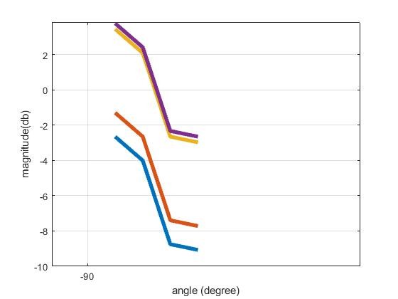
As you mentioned above, I also think that the number of sources is an important issue to solve in my case, in reference to the localization angles. As long as the number of sources is not well estimated, the `En = Ev(:,L+1:3)` in my code will display errors, hence the rest of the music code is adapted as follows:

    `SP= (En*a').*(a*En')./En.^2`

    `SP(iang,:) = abs((1./1-(SP(1,:))))`

and I get this result:

One question: If I reshape the code in several dimensions, will my result be displayed like yours in sinusoidal form or with peaks localization? Because It seems like my current result may not be correct and does not satisfy me at all.

When I describe the figure, I assume that the two users represent the two portions and individually emit their own characteristics. I don't know if this is correct. But it's just a brief interpretation in case the assumption is true.

Thank you for your clarification.

I don't know what your hardware setup is, but it is surprising to me that you talk about sound recordings and the speed of light. I would expect the speed of sound to be more relevant. However, since you got good results with beamforming, I guess what you have done is somehow correct.

There is no sense in thinking about algorithms to estimate the number of sources when you don't yet have an example working where the number of sources is known exactly.

Your equations didn't make sense to me. Please check that they have been typeset correctly.

I didn't understand your comments about reshaping the code.

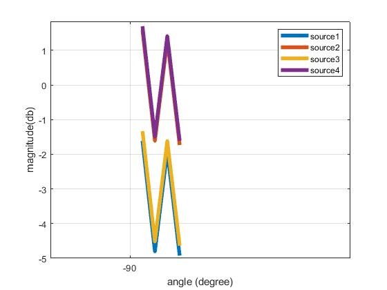
Your most recent graph is too small to read. It looks incorrect, but I can't read the legend to see what the 4 different lines represent.

Sorry, I was talking about the reshaping of the data in multiple dimensions. Because when I refer to the idea where I randomly generate the transmitted signal and the received signal, the data obtained are aligned in multiple dimensions, but my real data has one dimension, so if possible to reshape it in multiple dimensions.
To better clarify my work, here is my real signal generated from my smartphone:

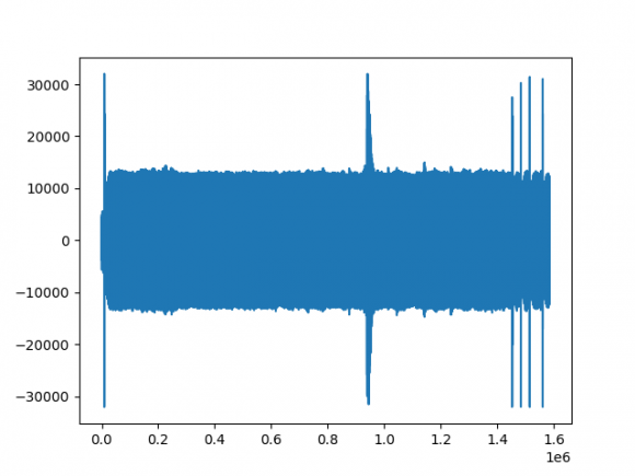
. I work only with a smartphone, with no extra device as support. FMCW is used as the transmit signal. I have two targets in my environment which represent my two sources (M=2), except other sources of reflection (maybe the wall, tools...). The exploiting data are those after the pre-processing.
The Music algorithm script is represented as follows:
%Music method
for iangl = 1:361
angle(iangl) = (iangl-180)/2
phim = degree_inradian*angle(iangl)
a = exp(-j*twp*d*cos(phim))'.
L = wave
En = EV(:,L+1:M)
SP(iangl) = (a*a')./(a*En'*En*a)
end
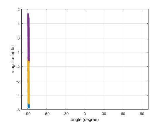
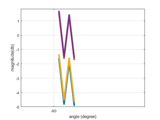
By incompatibility of dimensions I modified this part, to finally compile my data:
%Music method
for iangl = 1:361
angle(iangl) = (iangl-180)/2
phim = degree_inradian*angle(iangl)
a = exp(-j*twp*d*cos(phim))'.
L = wave
En = EV(:,L+1:M)
SP= (En*a').*(a*En')./En.^2
SP(iangl,:) = abs((1./1-(SP(1,:)))))
end
Unfortunately, I find this result,

 which seems to be incorrect, but indeed, I want to have more precision on it. And ask for help. I can inbox you to share my data and help me to solve this issue. How to successfully import my data in music algorithm or perhaps more algorithm to suggest.

Please attach your graphs and code for conventional beamforming.

It is only a small modification to convert that to use MUSIC.

Hi Sir, Sorry for being late. Here are my conventional beamforming code and figures. First I performed the pre-processing of my signal and later applied the MVDR algorithm for the conventional beamforming.

The first figure shows the signal after the pre-processing. The process has generated a lot of algorithms that I will not mention here. Below I have attached the MVDR code adapted to my signal and the result obtained.

                              `mvdr figure`

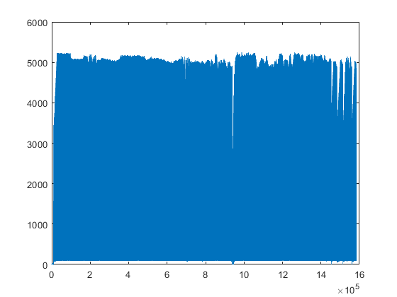
I think the result is correct?

So, how can I apply the Music from this result? and plot the spectrogram 1D or 2D?

```

% %Signal beamforming

%MVDR method
signal_data = abs(signal(5000:6000));
nbr_mics = 2;
nbr_snap = 200;
thetas = 30*pi/180;
center_frequency = 18000;
c =3e8;
lamda = c/center_frequency;
d = 0.5*lamda;%cell spacing
Is = zeros(nbr_mics,1);
for n = 1:nbr_mics
    Is(n) = exp(j*2*pi*(n-1)*d*sin(thetas)/lamda);

    Rxx = (signal_data.'*(signal_data.')')/nbr_snap;
    detaS = Is;
    Mvdr_algo(:,:,n) = inv(Rxx).*detaS(n).*inv(detaS(n)'.*inv(Rxx).*detaS(n));
end
%Linear array
p = -pi/2:pi/180:pi/2;
for jj = 1:1:length(p)
    w_scan = zeros(nbr_mics,1);
    scan = p(jj);
    for n = 1:nbr_mics
        w_scan(n) = exp(j*2*pi*(n-1)*d*sin(scan)/lamda);
    end
    Fmvdr(jj) = abs(Mvdr_algo(n)'.*w_scan(n));
    
end

% Figure
Fmax = max((Fmvdr));
Fa = Fmvdr./(Fmax);
Fa = 20*log10(Fa);
figure(1);
plot(180*p/pi,Fa,'b-')
xlabel('angle')

```

My data is so large that I share a fraction of it. You can check it out:

signal.mat

I can't really say much about the first figure. I guess it shows your signal is not all zeros, which is a good start.

Your second figure shows effectively all zeros (with some rounding errors). Therefore, I don't agree at all that it looks correct.

I tried to run your MATLAB code, but it fails. The variable "signal" is not defined. I tried loading the attached .mat file, but it doesn't contain any variable named "signal". I tried assigning one of the loaded variables to another variable named "signal" and running the script, but I get a different (also incorrect) result from what you showed above. It would be easier to help if you attached valid code.

I strongly suggest that you start with a working algorithm before trying to do anything with real-world signals. In other words, adapt my simple synthetic MUSIC example to work with MVDR. I recommend adapting my code and not using your code because your code is not working (and it isn't commented well, so it's difficult to debug).

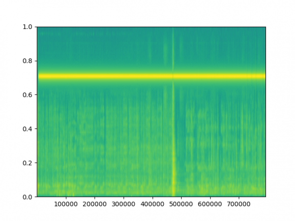
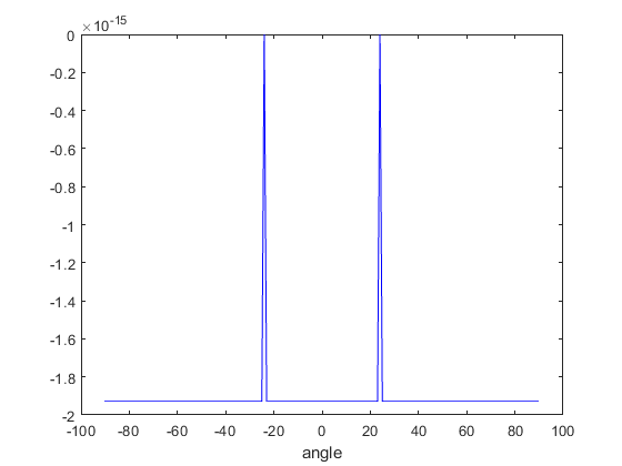
Hi Mr, sorry for the late reply. You can check out the result showing two peaks of AoA after beamforming. Now, I want to plot two-dimensional peaks and view them in the spectrogram domain representing the angle and range of the targets. The first picture shows the localization angle after beamforming, but I failed to reproduce the latter in the spectrogram as illustrated in the second figure. I want to plot something similar to " FM-Track: Pushing the Limits of Contactless Multi-target Tracking using Acoustic Signals" figure 6 (c). Can you provide some Matlab code?

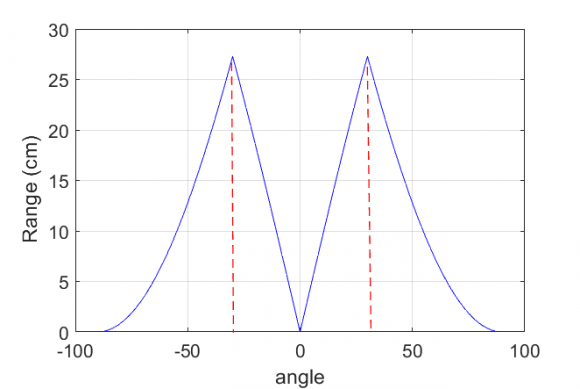
figure 1 p= -pi/2:pi/180/pi/2; plot(180*p/pi, abs(data)

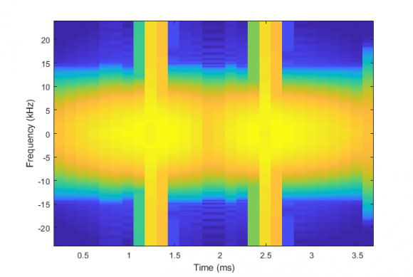
figure 2 pspectrum(data,48000,'spectrogram')

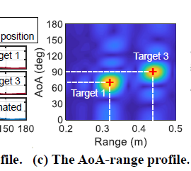
 figure 6(c) FM-Track article

my data: data.mat