I'm using a sliding RMS mechanism to compute RMS of a signal, i.e. with a window size of N, I add the squared value of the new sample x(n) to the running total while deducting the squared value of the x(n - N) sample and then performing a square root to get the RMS value.

This method works fine when a cycle's worth data in the signal under question lines up exactly with the length of the window. For ex,

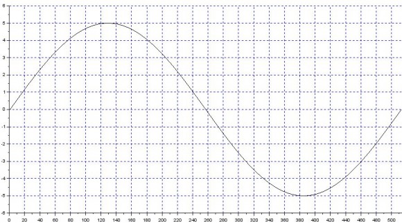
Let the window length N = 512, frequency of the signal = 100 Hz & sampling frequency = 51200 Hz.

With the above settings, every set of 512 samples would have a cycle's worth data of the signal & the computation works fine.

Now, the issue begins when the frequency of the signal deviates from 100Hz giving more or less number of samples in the same 512 samples window which throws off the accuracy of the sliding RMS algorithm.

This happens because the division by 512 to get the RMS, is no longer valid due to the fact that this particular cycle of the signal is getting complete before the end of the 512 samples window. However, the running squared total would already have the contributions from the previous samples which were divided by 512 while the samples of this cycle would require a different window length.

Is there a way to compensate for the addition/lack of samples due to the frequency drifts while using this technique?

Hi johnny_smith911. I spent 15 minutes trying to enter two MathJax equation in a reply for you, but I failed.  So I deleted my first reply and now I will try again by pasting JPG images of equations in my reply.

From your first paragraph it seems you are computing: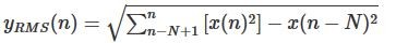

But then later in your post you mention a "division by 512."  The above expression contains no division. So we don't know what computations you are performing.  If I'm not mistaken, the following expression shows how to compute a 'sliding RMS':

I'm not sure what you're computing but I wonder if you're computing a value that's equal to an N-point RMS value only under the special condition that your input is a sinusoid having exactly N samples/cycle.

johnny_smith911, the above second yRMS(n) expression is not computationally efficient.  If your input signals have zero DC bias (zero-mean signals) I can give you a couple of different efficient ways to compute a 'sliding RMS' sequence.  Let me know by replying to this post of mine.

Hi Rick!  For your reference:

$$ y_{RMS}(n) = \sqrt{ \sum_{n-N+1}^n [x(n)^2] - x(n-N)^2 }  $$
$$ y_{RMS}(n) = \sqrt{\frac{1}{N} \sum_{n-N+1}^n x(n)^2 }  $$

$$ y_{RMS}(n) = \sqrt{ \sum_{n-N+1}^n [x(n)^2] - x(n-N)^2 } $$ $$ y_{RMS}(n) = \sqrt{\frac{1}{N} \sum_{n-N+1}^n x(n)^2 } $$

Hi Stephane,

   That is EXACTLY what I entered into the editor, except I only had one '$' at the beginning and one '$' at the end of the line of my MathJax characters. With only one '$' should my MathJax characters have been be ignored?  Thanks.

I totally understand the reason of your confusion.  For the blogs, one '$' is used for 'inline' equations, but it has caused trouble because when someone use twice the '$' in a post, like in: 'This cost $35 and this cost $36', Mathjax will interpret the content between the two '$' as TeX code and it doesn't look pretty.  

So for the forums, I have configured Mathjax so the inline equations delimiters are:

\( ... \)

I intend to port this improvement to the blogs eventually but it will require looking for all blog posts with Mathjax code and updating the delimiters...

Sorry for the confusion Rick.

Thanks Stephane!!

[-Rick-]

Hi Rick,

Thanks for your reply. Let me explain the algorithm that I'm using.

1. Keep acquiring samples until one full cycle is complete (using zero crossings to detect the completion).

2. Once a full cycle is obtained, get the window length.

3. Go through each sample in the window by adding the contribution of the current sample x(n) * x(n) / N while subtracting the contribution of the oldest sample(assume there was one full cycle before the start of this cycle) in the window x(n-N) * x(n-N) / N and obtaining a square root.

I guess this is similar to the 2nd method that you've mentioned with the difference that the samples from the previous cycle are involved & it's not just addition but subtraction is present as well.

This works fine if the window N has the same length in both the present & previous cycles. As this isn't the case & the lengths differ between cycles during frequency drifts, the process of addition & subtraction introduces errors which I'm not able to overcome. Please do note that RMS is needed on a sample by sample basis & not cycle by cycle basis.

Unfortunately, the input signal can contain DC offset at times & that can't be ignored.

johnny_smith911, it seems to me that you are performing the following:

where the above x(n) input sequence is your squared input samples, my 'D" is your 'N', and you're computing the square root of the output of my above diagram. The above is a "recursive running sum" operation and off the top of my head it seems like you are computing a "correct" instantaneous (sample-to-sample) RMS value.  The above is an efficient and equivalent version of the following "moving average" operation:

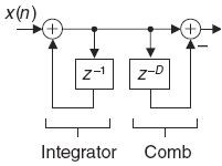
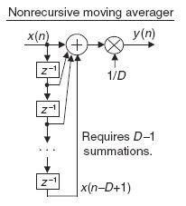
If you implement my second diagram (where my x(n) is your squared input samples), and perform the square root of its y(n) output sequence, I think you should obtain exactly the same output sequence that you computed using your method.  If that's true, then I believe you are computing correct RMS values.  (My two diagrams come from Chapter 10 of my DSP book. Notice that my second diagram has one fewer delay elements than my first diagram and that both networks must have their delay lines filled with valid data before their outputs are correct.)

But Fred Marshall brings up a beautiful point! For exactly one cycle of a sine wave, whose peak amplitude is A, the true RMS value will be A/sqrt(2).  The correctly-computed RMS value for a time interval more or less than exactly one cycle will be some correct value, but it will NOT be equal to A/sqrt(2).  johnny_smith911, is it possible that your computations are correct but they're merely different than what you expected?

Yes, I think both methods should give the same result & the second method should be computationally more efficient.

However, both these methods I believe, are plagued by the same problem. Let me explain with an example to make things a bit more clear.

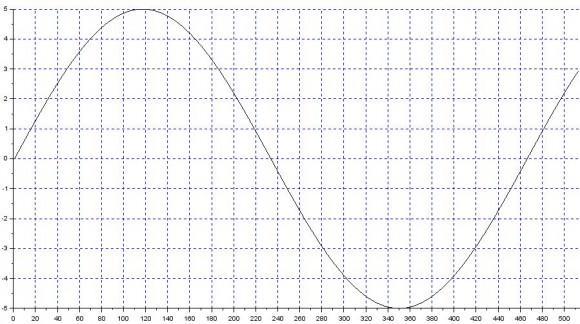
Lets say that our window length is N = 1000, sampling frequency Fs = 100,000 Hz & we have 2 cycles of the input signal under consideration. Let the 1st one have a frequency of 100Hz, i.e one full cycle in window 1 & let the 2nd cycle have a frequency of 180Hz meaning a full cycle in 55% of the window length or in other words a full cycle in just 555 samples in the 1000 samples window. The diagram below shows this.

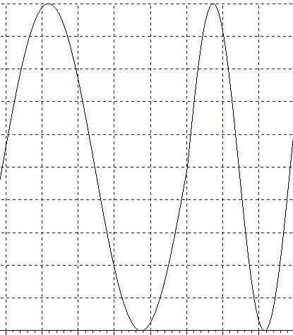
In case both cycles had 100Hz & we were to subtract the contribution of the oldest sample while adding the contribution of the newest sample while moving through the length of the 2nd cycle, there'd be no problem with the calculation because in both cases we'd have exactly 1000 samples for each cycle. This means, we'd be loosing 1000 samples while gaining 1000 new ones.

However, in the case shown above, the 1st cycle has 1000 samples while the 2nd one has ~555 samples. While computing the sliding RMS for the 2nd cycle, we only have 555 new samples but there are 1000 old samples for us to lose during the course of the entire cycle. Now, if we were to lose only 555 old samples, the remaining 445 would still remain in the running total thereby giving an error. This is with method 1 & I think method 2 will have the same problem but in a slightly different way.

The error itself would look like this.

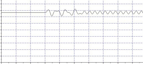
Notice how a ripple was introduced at the point where the frequency changes which continues to persist until the frequency deviation is present.

This is indeed an error & not merely different from what I expect cause the RMS of both these cycles irrespective of their frequencies, is still the same.

johnny_smith911, referencing your post that begins with "Yes, I think ...":

I can't interpret your two curves' time relationship because you did not label their horizontal axes. Also, I'm not able to understand what it means to "lose samples" or "gain samples."

When someone plots an "error" curve that curve usually represents the difference between two things. In your case can you tell us what

your error curve represents?  What did you subtract from what to produce that error curve?

johnny, I'm beginning to believe that your RMS computations are correct. That is, when you compute a single RMS output sample, you computing the correct RMS value for the previous N input samples.

The 1st cycle has a frequency of 100 Hz & fits perfectly in the N = 1000 samples window, i.e a full cycle of 100 Hz with nothing less or more fitting perfectly into the sliding RMS window of length N.

In the 2nd cycle, the magnitude is still the same but the signal now has a frequency of 180 Hz. This means, the cycle is complete is approx 555 samples (ignoring the fractional part) & does not perfectly fit the 1000 samples window.

Now, the RMS for cycle 1 is computed as follows(using method 1).

running_sum = running_sum + x(n) * x(n) / N

with n = 1 -> 1000

At the end of 1000 iterations, the RMS value of the signal is obtained. This is the 1st cycle of the signal, so the RMS will "grow" from 0 to the actual value.

For further cycles of the wave, i.e for each further sample (assuming all further cycles have the same magnitude), the RMS must be a constant value & not fluctuate like shown in the error diagram(note that in the diagram, the RMS is already a stable straight line. This is because the plot is taken not at the very 1st cycle but after several clean 100Hz cycles) irrespective of what the frequency is.

This is done by 

running_sum = running_sum + x(n) * x(n) / N

running_sum  = running_sum - x(n-N) * x(n-N) / N

where n = latest sample obtained & N = window length.

This simply means, we're dropping the contribution of the oldest sample while adding the contribution from the new one. All this works perfectly fine & we get a straight line for the RMS as long as each subsequent cycle fits in perfectly into the window length N. With 2 subsequent cycles which fit into 1000 samples, using the above algorithm means we're loosing a total of 1000 samples (1 at a time for each iteration) while gaining the contribution of 1000 new ones (again 1 at a time).

In other words, it means that we're slowly eliminating the contribution of the old cycle entirely while bringing in the new one.

However, as shown in the above example, this is not the case with cycle 2. Here, the cycle completed in ~555 samples instead of 1000. This gives an "effective" window length of 555 for cycle 2. Now, we cannot simply subtract the contribution of the oldest sample & add that of the new one. Why not? Cause we now have 2 "effective" window lengths. One for the 1st cycle with N1 = 1000 & N2 = 555. This time the iteration would have to run just 555 times.

In other words, we're not eliminating the contribution of all the samples of the previous cycles while accommodating the new one & at the end of 555 iterations, we still have the contribution of 445 samples from the previous cycles although we have completed covering this new cycle.

This introduces the ripple-like error in the calculation. Hope this clears things a bit.

If you know your new frequency (after deviation) then resize window.

If you don't know about new frequency then I believe you have to increase window size to an acceptable resolution for the deviation range.

Kaz

Hi Kaz,

I do know the new frequency after the deviation & yes, I do resize the window. However, this is just one part of the problem(albeit the easy one).

The other part is that, since this is a sliding RMS mechanism, I need RMS values sample by sample & not cycle by cycle. This means, after I gather samples for a full cycle, I go through each sample computing the RMS by adding the contribution of the current sample x(n)*x(n)/N while subtracting the contribution of the oldest sample in the window x(n-N)*x(n-N)/N and obtaining a square root.

This works fine if the window N has the same length in both the present & previous cycles. As this isn't the case & the lengths differ between cycles during frequency drifts, the process of addition & subtraction introduces errors which I'm not able to overcome.

so basically you are concerned about the transition section say from f1 to f2.

In that case I assume some feedback mechanism may do. I am not sure how but will think about it.

or try change window size gradually from w1 to w2

Kaz

Exactly. Some sort of compensation needs to be done while shifting from the old cycle to the new one to account for the difference in the window lengths while subtracting the contributions of the samples from the old cycle.

I've tried something similar to what you said, i.e. gradually change the window length but that didn't work well & the errors were still there. If the frequency difference between the 2 cycles is quite big (say almost 2 times), you can see quite a significant error.

I am thinking of continuous phase detection using an NCO to decompose signal to I/Q (relative to a fixed nco frequency) then use the I/Q result to adjust window size with some scaling.

Perhaps I'm missing something here...

The *usual* RMS measure of a sinusoid starts with the sinusoidal amplitude as in:

A*sin(wt) and the only thing of concern is "A" if one knows that they're dealing with a sinusoid in the first place.

But, it appears that you're sampling the entire A*sin(wt).

Then, in addition, you're taking but a single period of sin(wt).  It's no wonder that this causes trouble in meeting your apparent objective.  Imagine if you took 1.5 periods.  The RMS value of that particular "waveform" or shape has a large DC component which will be part of the RMS value you're computing.  

I would suggest that you start with the integral equation for rms:

           b   

1/(b − a) int |f(t)|^2 dt

           a

Converting this to a sum is easy enough.

My point is that the definition of f(t) is important to the outcome.  If f(t) is sin(wt) and the range a to b is some non-integer number of periods then the rms value will be what it is - but not the same as for a single period.

Hi Fred,you are right about rms formulas predefined for some known ideal waveforms.

The OP - I believe - wants to measure it in running mode rather than calculate it, just like averaging any other signal using Running Average filter.

kaz,  Thanks.  

I then still have to worry about what does RMS mean after all?  Or, why do we measure it? One definition (which I don't endorse or deny) is "the equivalent DC (constant) voltage value that gives the same effect.  And, the latter part is stated to mean "the same average power dissipation in a resistive load".

That said, it suggests a time frame over which it's measured.  Surely we've all looked at an RMS meter connected to a varying signal and have seen the values change.  So we're used to not expecting it to be "a number for all time".  

I think it's fair to say that the time span has to be "suitably long".

In this case, as was proposed, it's just not long enough to meet that standard.  We could then ask:

"If I want to measure the RMS value of a pure sinusoid by squaring, integrating, averaging and taking the square root, then how long does the record have to be to reach x% accuracy?"  That question can be answered. 

But the OP said he wants the RMS value on a sample-by-sample basis and would add a sample and drop a sample at each output sample.  And, the frequency is varying.  I would suggest that the analysis window is too short to accomplish this feat - and therin lies the problem.  

Maybe there should be a window of 1 sample.  I exaggerate but it makes the point doesn't it?  You can have the RMS value of *the sinusoidal part* or you can have the instantaneous RMS value of each sample which ignores the waveshape altogether.  As the analysis window goes from infinite or "large enough" down toward 1 or a few periods of the sinusoid then the outputs will vary accordinly - even though "correct".  Only by tuning the analysis can one capture a single sinusoidal period and then use other assumptions.  

I guess that's the choice.  Whether one is doing all the additions each time or is adding and dropping samples isn't the issue here I believe.

Indeed a precision running RMS algorithm as required by op is very extreme case but it could be part of academic research or some unknown corners of a control system. 

Even a given settled frequency will have some jitter or start from any phase. So the focus on frequency transition window sounds like an overkill and assumes that signal is perfect at f1 and f2 and at transition from f1 to f2. But we need to know the purpose in order to say "please, don't go that far"