i've started reading dspguide.com and came across through this.

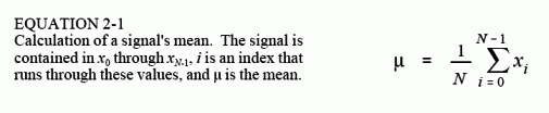
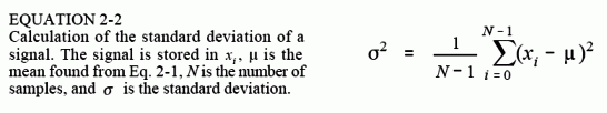
This method of calculating the mean and standard deviation is adequate for many applications; however, it has two limitations. First, if the mean is much larger than the standard deviation, Eq. 2-2 involves subtracting two numbers that are very close in value. This can result in excessive round-off error in the calculations. Second, it is often desirable to recalculate the mean and standard deviation as new samples are acquired and added to the signal. We will call this type of calculation: running statistics. While the method of Eqs. 2-1 and 2-2 can be used for running statistics, it requires that all of the samples be involved in each new calculation. This is a very inefficient use of computational power and memory.

how did the author conclude that if mean is larger than standard deviation then x[i] and μ are very close.

and how does the round-off error occur in the calculations?

>and how does the round-off error occur in the calculations?

Read What Every Computer Scientist Should Know about Floating-Point Arithmetic

>how did the author conclude that if mean is larger than standard deviation then x[i] and μ are very close.

This is one of the properties of mean and standard deviation; if you calculate \( k_i = \dfrac{x_i - \mu}{\sigma} \) then a very large fraction of \( k_i \) have \( |k_i| < 6 \) (in other words, the vast majority of data points are within 6 standard deviations of the mean).

edit: regarding round-off and this specific calculation, your best bet is to read Knuth's The Art of Computer Programming vol 2, which talks about Welford's algorithm that I discussed in one of my articles.

You mean \( \left| k_i \right| < 6\sigma \).  Otherwise -- yes, you beat me to it, and said exactly what I would have said.

No, what I posted was correct; \( k_i \) is normalized to represent the number of standard deviations away from the mean.

Whoops.  I missed that.  Sorry.

>and how does the round-off error occur in the calculations?

jms_nh's link answers this, but the short answer is that floating-point numbers are subject to the "subtracting two big numbers to get a little number is inaccurate" rule.  What constitutes "big" and "little" and "inaccurate" are subject to the problem at hand, so it's good to understand the underlying math -- which, I trust, is in the referenced paper.

The way I visualise this issue (for electronic signals at least) is that the mean is the "dc" offset while standard of deviation is the "AC" mean. 

Thus if mean (i.e. DC offset) is very high it will waste a lot of bit resolution at implementation. 

The mean can be subtracted first to remove dc offset. Then all resolution becomes available for AC mean. I wonder if it is useful then to add the DC offset back.

However, DC can be an important signal component. If the signal under test is a direct demodulated version of an RF signal, then for AM modulated signals (e.g. ILS, VOR, and similar), the DC represents the carrier level (essentially the inverse of the generating function). If the demodulation is done in a receiver with AGC, then the DC represents the receiver's AGC reference level and is not related to the carrier level, so "extracting" the carrier's level must be done by calculating the AGC gain based on the receiver's transfer function or other means related to the receiver design (e.g. log amp).

Note that when the signal's DC representing carrier level is a critical signal component, then any real DC offsets are errors and must be estimated and removed to determine the true RF carrier level. In that case, each signal component should be processed separately for stddev and not as an ensemble or group (think apples and oranges). In fact, for an ILS (Instrument Landing System) signal, the difference in the 90 and 150 Hz AM components represents a plane's azimuth (horizontal) or glidepath (vertical) position relative to the runway's centerline and touchdown point, respectively. So in that case, errors in the 90 and 150 Hz components must be estimated separately.

>how did the author conclude that if mean is larger than standard deviation then x[i] and μ are very close.

σ^2 = E{(x - μ)^2}, where E{x} = μ.

μ >> σ^2, for example μ > 10*σ^2 =>  E{(x - μ)^2} < μ/10.

The relationship   E{(x - μ)^2} < μ/10 suggests that the difference

(x - μ)^2  has   μ/10 as a superior bound. 

You ask, how did the author reach this conclusion:

First, if the mean is much larger than the standard deviation, Eq. 2-2 involves subtracting two numbers that are very close in value.

You start with a large mean value and a small standard deviation.  Picturing this, the x[i] must all be near the mean so they are both large numbers and nearly equal.  So, the difference is going to be subject to errors.  That's all....

Now, you may want to ask: Why would the difference be subject to errors and that's the point that jms_nh has made I believe.

I'm an old-time embedded guy. I tend to automatically see problems from an embedded perspective and since the workproduct of many of these articles is destined for embedded applications or the like, these thoughts may be helpful. I have done lots of "math" using (underpowered) 8 and 16 bit uCs with only 64 Kbytes of address space where floating point was not an option. I typically use "binary point" numbers (an implied binary point in native data sizes) to accommodate issues like not having to normalize numbers (e.g. to make two numbers have the same characteristic so they can be added/subtracted). Much of my code uses P. J. Plauger's sage advice: keep data in it's rawest form for as long as possible before converting to its final form (e.g. scaling to engineering units).

With that as prelude, let's say that the final value being calculated originates from an A/D measurement and that this then gets massaged with additional scaling, etc. before its final form which is then typically plugged into a formula (e.g. stddev). It can be advantageous to rewrite the code to maintain the data in its raw form and perform a stddev on THAT. This allows the use of sufficiently sized integer math (8/16/32/64 etc. bits) to avoid scaling and (most) calculation induced noise in the measurement plus it can be really fast if using the micro's native integer operations. This scheme is ideal for any kind of sliding windowed calculations like stddev. Once the stddev in raw form is calculated, the values can be scaled as desired to minimize truncation errors (i.e. noise) induced by any normalization operations. This can be of benefit even for processors with native floating point operations that are as fast as native integer operations. For many RISC processors, data transfers larger than the native bus width can really be slow, so keeping the raw data in integer format can speed up operations too.

If corrections are needed, it may be possible (or necessary) to do those at the integer level to be sure that all "raw" data are in the "same units". Corrections might include A/D zero and gain corrections to compensate for various drifts (temperature, aging, supply, etc.) generally using measurements of a "known good" (by definition) Voltage reference and analog ground (the working assumption is that the Voltage reference drifts less than everything else!). So the gain/offset adjustment should be done to the uncompensated raw data to derive the compensated raw data before being used in the window processing. Ignoring these errors, (especially if it is supposed to work from -20degC to +85degC as much of my work does) is done at your peril. Be sure that the required accuracy is known (not just resolution). Use datasheet information to derive an error model for the hardware configuration. These errors can be more important than just "getting the math right", which is assumed.

Modeling an algorithm in something like MATLAB is nice to verify the basic algorithm, but getting that converted and optimized for embedded use can be a much bigger challenge.