I recently inquired about A & C weighted filters.  While researching how to generate A & C filters using MatLab (which I know absolutely nothing about.  Sadly, I am just borrowing code), I found code that generates coefficients for these weighted filters.  They all generate output from bilinear transform.  In my research I found that the output from the bilinear transform can be converted to second order sections using tf2sos, which is exactly what I want.  One of my sticking points is that when I generated those second order sections (a0, a1, a2, b0, b1, b2), the b0 did not equal 1 as I expected.

The usage of tf2sos would be perfect but what I found is that values generated create 6 coefficients (a0, a1, a2, b0, b1, b2) , however what I need is 5 (a0, a1, a2, b1, b2).  I do know naming conventions differ but I am still referring to the same thing whether you call them a or b.  What I understand is that a normalization of required to make the b0 = 1 in (a0, a1, a2, b0, b1, b2), leaving the final result as (a0, a1, a2, b1, b2).

How do I get to the point where I can obtain the 5 coefficients

[b,a] = bilinear(NUM,DEN,Fs);
sos = tf2sos(b,a);
printf('%0.16f\n',sos);

(robert bristow-johnson)https://www.dsprelated.com/showthread/comp.dsp/693...

https://www.dsprelated.com/showcode/214.php
https://www.dsprelated.com/showcode/215.php

Thank you,

MrE

Divide every coefficient by \(b_0\), i.e. \(a_0' = \frac{a_0}{b_0}\), \(b_1' = \frac{b_1}{b_0}\), etc..  The resulting \(b_0'\) will be equal to 1.  Assuming the routine does what's expected, you should be good to go with the new set of coefficients.

Excellent.  I thought I'd seen this before (dividing everything by b0).

>>Assuming the routine does what's expected...

You're absolutely right.  I really dont know.  Those second order section coefficients really looked odd. I'm hoping to test this out tonight and practically praying for a mini-miracle.

Hi,

For a biquad, the feedback coeffs are [1 a1 a2] and the feedforward coeffs are [b0 b1 b2].  The a0 coefficient does not appear explicitly in the filter structure.  The tf2sos *may* be normalizing the b's such that the gain at dc is 1.0 --  which may be why b0 is not equal to one.

For more on lowpass biquads, see my recent post:  https://www.dsprelated.com/showarticle/1137.php

regards,

Neil

I hadn't considered there may be something else occurring with b0.  I'll check out your article.  Unfortunately, I am math challenged (gleaning rather than consuming) but I continue to try to understand.

D'oh.  Too much Scilab -- Scilab just gives you transfer functions, not anonymous arrays of coefficients.

After a lot of thinking and reading, I determined that I misunderstood the array output order of the ts2sos function.  I converted the output order to the order which I planned to use.  Even though I learned the naming convention differently, for clarity, I will stick with [b0, b1, b2, 1, a1, a2] where a0 = 1.

All looked like it was going well until I produced the output and saw that start around 6300Hz using a 44100 sampling frequency (48000Hz sampling was not much difference)things start to go awry.  My test frequencies, at 1/3 octave frequencies, has as much as 27 decibel difference.  I apply a 2.76234698295594 offset to compensate to 0.0 db at 1000Hz. Is this what I should expect.  Just in case it matters, I am using Octave online https://octave-online.net/ to produce get the biquad coefficients.

Thank you,

MrE

https://www.dsprelated.com/showcode/214.php

%Sampling Rate
%Fs = 48000;
Fs = 44100;

%Analog A-weighting filter according to IEC/CD 1672.
f1 = 20.598997;
f2 = 107.65265;
f3 = 737.86223;
f4 = 12194.217;
A1000 = 1.9997;
pi = 3.14159265358979;
NUM = [ (2*pi*f4)^2*(10^(A1000/20)) 0 0 0 0 ];
DEN = conv([1 +4*pi*f4 (2*pi*f4)^2],[1 +4*pi*f1 (2*pi*f1)^2]);
DEN = conv(conv(DEN,[1 2*pi*f3]),[1 2*pi*f2]);

%Bilinear transformation of analog design to get the digital filter.
% bilinear(NUM,DEN,1/Fs) — where 1/Fs is what Octave expects vs MatLab FS

[b,a] = bilinear(NUM,DEN,1/Fs);
sos = tf2sos(b,a);
printf('%0.16f\n',sos);

%output of tf2sos

0.2557411252042576
1.0000000000000000
1.0000000000000000
-0.5114387219173979
-2.0001702052850550
2.0000000000000018
0.2556976004164214
1.0001702197743114
1.0000000000000016
1.0000000000000000
1.0000000000000000
1.0000000000000000
-0.1405360824207118
-1.8849012174682307
-1.9941388812268852
0.0049375976155401
0.8864214718516013
0.9941474694047874

reordered array output for my function [b0, b1, b2,1, a1, a2]

ax = [0.2557411252042576,     -0.5114387219173979,     0.2556976004164214,     1.0000000000000000,     -0.1405360824207118,     0.0049375976155401]
ax = [1.0000000000000000,     -2.0001702052850550,     1.0001702197743114,     1.0000000000000000,     -1.8849012174682307,     0.8864214718516013]
ax = [1.0000000000000000,     2.0000000000000018,     1.0000000000000016,     1.0000000000000000,     -1.9941388812268852,     0.9941474694047874]

indx     freq     expectedDB         coeffResultDB         error (expectedDB-coeffResultDB)

1.    20.0    -50.394855    -48.395002    -1.999854
2.    25.0    -44.820693    -43.027185    -1.793509
3.    31.5    -39.529064    -37.922292    -1.606772
4.    40.0    -34.539447    -33.105356    -1.434091
5.    50.0    -30.275178    -28.981509    -1.293669
6.    63.0    -26.223024    -25.061738    -1.161285
7.    80.0    -22.397865    -21.367662    -1.030203
8.    100.0    -19.145152    -18.231199    -0.913954
9.    125.0    -16.189851    -15.386256    -0.803595
10.    160.0    -13.244525    -12.551357    -0.693168
11.    200.0    -10.847252    -10.242894    -0.604357
12.    250.0    -8.675022    -8.151094    -0.523929
13.    315.0    -6.643962    -6.199715    -0.444247
14.    400.0    -4.774080    -4.414373    -0.359708
15.    500.0    -3.247992    -2.972832    -0.275159
16.    630.0    -1.908628    -1.726412    -0.182216
17.    800.0    -0.794769    -0.709600    -0.085169
18.    1000.0    0.000000    0.000000    -0.000000
19.    1250.0    0.576176    0.500284    0.075892
20.    1600.0    0.993092    0.848173    0.144919
21.    2000.0    1.201699    1.005786    0.195914
22.    2500.0    1.271104    1.016600    0.254504
23.    3150.0    1.201781    1.605448    -0.403667
24.    4000.0    0.964229    0.627635    0.336594
25.    5000.0    0.555465    0.162086    0.393379
26.    6300.0    -0.113951    8.166050    -8.280001
27.    8000.0    -1.144507    0.656249    -1.800757
28.    10000.0    -2.488333    9.699220    -12.187553
29.    12500.0    -4.249819    5.350868    -9.600686
30.    16000.0    -6.700912    4.426299    -11.127211
31.    20000.0    -9.340763    17.277129    -26.617892

I noticed there is some Matlab code for the A-weighted filter in a DSPrelated post from 2011:

https://www.dsprelated.com/showcode/214.php

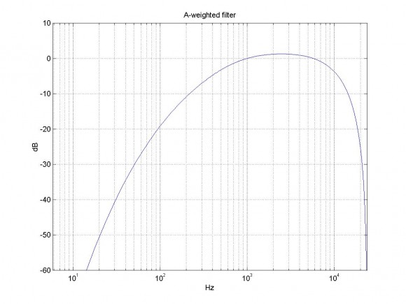
Here is the code, with the resulting coeffs.  I added plotting.  See figure below.  Note this is a 6th order filter.

%Aweighted.m

%Sampling Rate

Fs = 48000;

%Analog A-weighting filter according to IEC/CD 1672.

f1 = 20.598997;

f2 = 107.65265;

f3 = 737.86223;

f4 = 12194.217;

A1000 = 1.9997;

pi = 3.14159265358979;

NUM = [ (2*pi*f4)^2*(10^(A1000/20)) 0 0 0 0 ];

DEN = conv([1 +4*pi*f4 (2*pi*f4)^2],[1 +4*pi*f1 (2*pi*f1)^2]);

DEN = conv(conv(DEN,[1 2*pi*f3]),[1 2*pi*f2]);

%Bilinear transformation of analog design to get the digital filter.

[b,a] = bilinear(NUM,DEN,Fs)

% plot response

[h,f]= freqz(b,a,4096,Fs);

H= 20*log10(abs(h));

semilogx(f,H),grid

axis([0 Fs/2 -60 10])

xlabel('Hz'),ylabel('dB')

title('A-weighted filter')

b =0.2343 -0.4686 -0.2343 0.9372 -0.2343 -0.4686 0.2343

a =1.0000 -4.1130 6.5531 -4.9908 1.7857 -0.2462 0.0112

I used the same code base. https://www.dsprelated.com/showcode/214.php

I believe that if my method for determining the error rate were incorrect then it would have shown up previously in the last few years.

I cant say that I understand the graph, however what I applied pure tones to the filter in 1/3 octaves and determined the error in decibels.  A less than 1db error is what I'm aiming for.  In my previous post using the derived coefficients, we start out with a ~2db error and start getting better until we get to 6300Hz with an 8db error to ~27db error as 20KHz.  If that is the actual error difference that I should expect, then I just have to try something different.

MrE

Hello,

You've likely already found the issue with your script-file, but the third argument to the "bilinear" function should be "Fs" not "1/Fs".  With this change your code produces the same A-weighted response generated by the code offered by NEIROBER.

Using the "b" and "a" coefficients and the TF2SOS function, the frequency-magnitude response of the SOS matrix can be plotted.

sos = tf2sos(b, a, 'up', 'none');
figure;
     [h, f]=freqz(sos, 4096, Fs); plot(f, 20*log10(abs(h))); grid on; shg;
     set(gca, 'XScale', 'log');

The values in the SOS matrix are,

sos =


   0.234301792299513   0.468603584599026   0.234301792299513   1.000000000000000  -1.893870494746436   0.895159769115844
   1.000000000000000  -2.000230909187332   1.000230935849392   1.000000000000000  -1.994614455969653   0.994621706990548
   1.000000000000000  -1.999769090812668   0.999769117469660   1.000000000000000  -0.224558458059779   0.012606625271547

Michael.

>> MichawelRW wrote:  You've likely already found the issue with your script-file, but the third argument to the "bilinear" function should be "Fs" not "1/Fs".

The use of "1/FS" was intentional because I do not have access to MatLab but rather I have been utilizing Octave online (https://octave-online.net) and the tf2sos function utilizes the period instead of the sampling rate in the third argument but otherwise is the same.

MrE

Very good.