A Simpler Goertzel Algorithm

In this blog I propose a Goertzel algorithm that is simpler than the version of the Goertzel algorithm that is traditionally presented DSP textbooks. Below I very briefly describe the DSP textbook version of the Goertzel algorithm followed by a description of my proposed simpler algorithm.

The Traditional DSP Textbook Goertzel Algorithm

The so-called Goertzel algorithm is used to efficiently compute a single mth-bin sample of an N-point discrete Fourier transform (DFT) [1-4]. The traditional DSP textbook version of the Goertzel algorithm is implemented using the network shown in Figure 1.

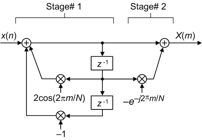
Figure 1: Traditional DSP textbook Goertzel network.

The ‘m’ variable in Figure 1 is the index of the single DFT bin sample being computed where m = 0,1,2,…,N-1, N is the DFT size, and the X(m) output is the desired mth-bin DFT sample. The z-domain transfer function of the Figure 1 network is:

$$H_1(z) = {1-e^{-j2{\pi}m/N}z^{-1}\over 1-2cos(2{\pi}m/N)z^{-1}+z^{-2}}.\qquad\qquad\qquad(1)$$

The processing steps used to compute the complex-valued X(m) output sample in the Figure 1 network are as follows:

1) Apply an N-sample x(n) input sequence to the network performing the Figure 1 Stage# 1 computations N times.

2) Shift the data samples downward through the two delay elements.

3) Apply a zero-valued input sample to the network’s input and perform the Figure 1 Stage# 1 computations one more time.

4) Perform the Figure 1 Stage# 2 computations one time to obtain the desired X(m) sample.

The Proposed Simpler Goertzel Algorithm

We can eliminate the above traditional Figure 1 processing Steps 2) and 3) by using the network shown in Figure 2.

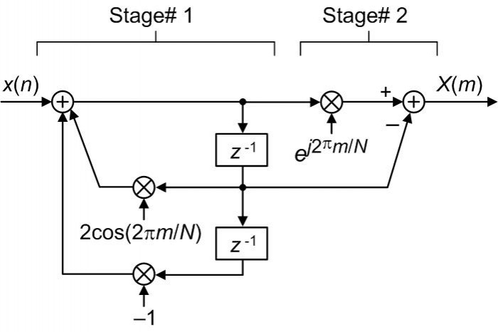
Figure 2: Proposed simpler Goertzel network.

The z-domain transfer function of the Figure 2 network is:

$$H_2(z) = {e^{j2{\pi}m/N}-z^{-1}\over 1-2cos(2{\pi}m/N)z^{-1}+z^{-2}}.\qquad\qquad\qquad(2)$$

The simpler processing steps used to compute the complex-valued X(m) output sample in the Figure 2 network are as follows:

1) Apply an N-sample x(n) input sequence to the network performing the Figure 2 Stage# 1 computations N times.

2) Perform the Figure 2 Stage# 2 computations one time to obtain the desired X(m) sample.

A Noteworthy Aspect Regarding the Original 1958 Goertzel Algorithm

It is interesting to note that the traditional Figure 1 DSP textbook version of the so-called Goertzel algorithm does not implement the processing originally proposed by Gerald Goertzel in his 1958 paper [5].

I make the above claim because in Gerald Goertzel’s original paper the input data sequence must be reversed in order to produce the desired a(k) data sequence as indicated by his decrementing time-domain index ‘k’ shown in Figure 3.

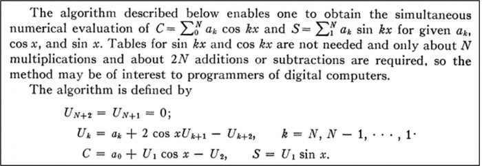
Figure 3: The original algorithm proposed by G. Goertzel in  1958. [Reproduced from [5] without permission.]

At this point I’ll also state that I believe the lower limit of the ‘S’ summation in the text of Figure 3 should be zero rather than one.

Conclusions

I briefly described the Figure 1 network and processing steps of the traditional DSP textbook version of the so-called Goertzel algorithm. (I refer to that textbook algorithm as “so-called” because it does not implement the original algorithm proposed by G. Goertzel in his 1958 paper.) Then I proposed the Figure 2 network and processing steps of a simpler Goertzel algorithm.

My proposed algorithm is only slightly computationally simpler than the traditional algorithm but it does eliminate the tradition algorithm’s cumbersome processing Steps 2) and 3).

References

[1] S. Mitra, "Digital Signal Processing", Fourth Edition, McGraw Hill Publishing, 2011, pp. 618-620.

[2] J. Proakis and D. Manolakis, "Digital Signal Processing-Principles, Algorithms, and Applications", Third Edition, Prentice Hall, Upper Saddle River, New Jersey, 1996, pp. 480-481.

[3] A. Oppenheim, R. Schafer, and J. Buck, "Discrete-Time Signal Processing", Second Edition, Prentice Hall, Upper Saddle River, New Jersey, 1996, pp. 633-634.

[4] R. Lyons, “Understanding Digital Signal Processing”, 3rd Ed., Prentice Hall, Upper Saddle River, New Jersey, 2011, pp. 738–740.

[5] G. Goertzel, “An Algorithm for the Evaluation of Finite Trigonometric Series” The American Mathematical Monthly, Vol. 65, No. 1, Jan. 1958, pp. 34-35

Sign in