Digital State Variable Filters

• Audio DSP
• Academia / Research
• Design Methodolgies

A classic analog filter is the so-called "state variable filter". This blog covers realization of a continuous-time second-order lowpass filter as a state-space model which is then digitized via both forward and backward Euler schemes to produce the so-called Chamberlin form of a digital resonator (which has desirable numerical properties). Finally, the Faust form of the resonator is derived.

Normalized Second-Order Continuous-Time Lowpass Filter

The transfer function of a normalized second-order lowpass can be written as

where the normalization maps the desired -3dB frequency  to 1, i.e.,

and the ``quality factor'' Q is defined as

where is a convenient definition for bandwidth in radians per second, given by minus the real part of the complex-conjugate pole locations  and  in the  plane:

Here we assume , so that the poles have nonzero imaginary parts.

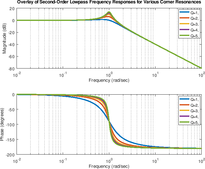
A second-order Butterworth lowpass filter is obtained for . Larger Q values give the ``corner resonance'' effect often used in music synthesizers.

Bode Plots for Second-Order Butterworth Filters

Filters of this type are nicely viewed in a Bode plot which shows the magnitude frequency response (in dB) versus a log frequency axis.  In matlab we can say, for example,

sys = tf(1,[1,sqrt(2),1]);

bode(sys);

to see the frequency response of our normalized second-order Butterworth lowpass filter.

Note that our lowpass is easily converted to a bandpass or highpass filter by changing the transfer-function numerator from 1 to  or , respectively:

bode(tf([0 0 1],[1,sqrt(2),1])); % lowpass
bode(tf([0 1 0],[1,sqrt(2),1])); % bandpass
bode(tf([1 0 0],[1,sqrt(2),1])); % highpass
bode(tf([1 0 1],[1,sqrt(2),1])); % notch

These frequency responses are shown below:

Figure 1: Overlay of normalized second-order Butterworth lowpass, bandpass, highpass, and notch filters.

$$y(t) = k_0 + \sum_{n=1}^{\infty} \int_{-\infty}^{\infty}\cdots \int_{-\infty}^{\infty}k_n(t_1,t_2,\ldots,t_n)x(t-t_1)x(t-t_2)\cdots x(t-t_n)dt_1dt_2\cdots dt_n$$

Sign in