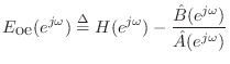
The equation error is defined (in the frequency domain) as
By comparison, the more natural frequency-domain error
is the so-called output error:
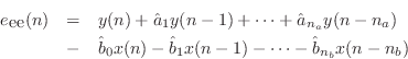
The names of these errors make the most sense in the time domain. Let
 and
and  denote the filter input and output, respectively, at time
 . Then the equation error is the error in the difference equation:
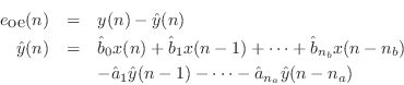
while the output error is the difference between the ideal and approximate
filter outputs:
Denote the  norm of the equation error by
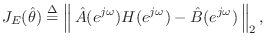 |
(I.11) |
where
![$ \hat{\theta}^T = [\hat{b}_0,\hat{b}_1,\ldots,\hat{b}_{{n}_b}, \hat{a}_1,\ldots, \hat{a}_{{n}_a}]$](http://www.dsprelated.com/josimages_new/filters/img2401.png)
is the
vector of unknown filter coefficients. Then the problem is to minimize
this norm with respect to

. What makes the equation-error so easy to
minimize is that it is
linear in the parameters. In the time-domain
form, it is clear that the equation error is linear in the unknowns

. When the error is linear in the parameters, the sum of
squared errors is a
quadratic form which can be minimized using one
iteration of
Newton's method. In other words, minimizing the
norm of
any error which is linear in the parameters results in a set of linear
equations to solve. In the case of the equation-error minimization at
hand, we will obtain

linear equations in as many unknowns.
Note that (I.11) can be expressed as
Thus, the equation-error can be interpreted as a
weighted output
error in which the frequency weighting function on the unit circle is
given by

. Thus, the weighting function is determined
by the filter
poles, and the error is weighted
less near the
poles. Since the poles of a good
filter-design tend toward regions of
high spectral energy, or toward ``irregularities'' in the
spectrum, it is
evident that the equation-error criterion assigns less importance to the
most prominent or structured spectral regions. On the other hand, far away
from the roots of

, good fits to
both phase and magnitude can
be expected. The weighting effect can be eliminated through
use of the
Steiglitz-McBride algorithm
[
45,
78] which iteratively solves the weighted
equation-error solution, using the canceling weight function from the
previous iteration. When it converges (which is typical in practice), it
must converge to the output error minimizer.
Next Section: Error Weighting and Frequency WarpingPrevious Section: Examples