


Why Time-Domain Zero Stuffing Produces Multiple Frequency-Domain Spectral Images
This blog explains why, in the process of time-domain interpolation (sample rate increase), zero stuffing a time sequence with zero-valued samples produces an increased-length time sequence whose spectrum contains replications of the original time sequence's spectrum.
Background
The traditional way to interpolate (sample rate increase) an x(n) time domain sequence is shown in Figure 1.
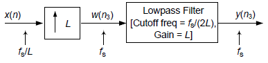
Figure 1
The '↑ L' operation in Figure 1 means to insert L–1 zero-valued samples between each sample in x(n), creating a longer-length w(n3) sequence. (The sample rate of the x(n) input is fs/L samples/second.) To the end of that longer sequence we append L–1 zero-valued samples. Those two steps are what we call "upsampling." Next, we apply the upsampled w(n3) sequence to a lowpass filter whose output is the interpolated y(n3) sequence. We formally refer to interpolation as the two-step process of upsampling followed by lowpass filtering.
An Example
An example of the Figure 1 process is given in Figure 2. In this example the input x(n) time sequence is the sum of two sine waves. The discrete Fourier transform (DFT) of x(n) is X(m). Because the x(n)sequence comprises sine waves, the real parts of X(m) are zero-valued. As such, we'll plot the imaginary parts of the X(m) spectral samples as the Imag[X(m)] sequence shown on the right side of Figure 2(a).
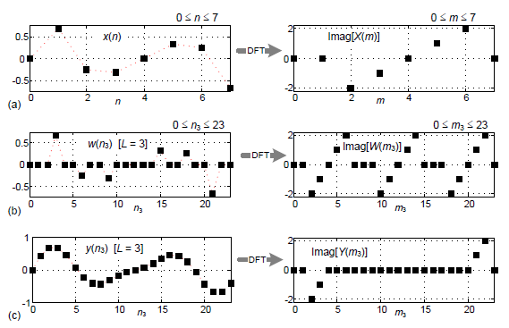
Figure 2
Upsampling x(n) by L = 3 produces the w(n3) sequence shown at the left side of Figure 2(b). The imaginary parts of the W(m3) DFT spectral samples are represented by the Imag[W(m3)] sequence shown on the right side of Figure 2(b). Notice that the Imag[W(m3)] sequence contains replications of the Imag[X(m)] spectral samples.
Our Question
The question that occurs to people when they first study the topic of time-domain interpolation (the question answered in this blog) is,
"Why does inserting zero-valued samples in x(n) to produce w(n3) result in a W(m3) spectrum containing replications of the original X(m) spectral samples?"
An Intuitive Answer
One answer to our question involves recalling how the DFT of several periods of a periodic time signal is a discrete Fourier series (DFS). That is, a DFS containing non-zero-valued spectral samples separated by zero-valued spectral samples. In our Figure 2(b) case we exchange the traditional DFS time and frequency domains. The inverse DFT of several periods of a periodic W(m3) spectrum results in a w(n3) time sequence containing non-zero-valued time samples separated by zero-valued time samples.
OK, given that hand-waving intuitive answer we now present an alternate answer to our question by way of an example.
An Answer By Way of Example
An alternate answer to our question comes from our realization that the two sequences in Figure 2(b) are Fourier transform pairs. That is, we can show that the inverse DFT of the Imag[W(m3)] sequence really does produce the zero-valued samples in the w(n3) time sequence. For example, let's show why the w(1) and w(2) samples are zero-valued as shown on the right side of Figure 3.
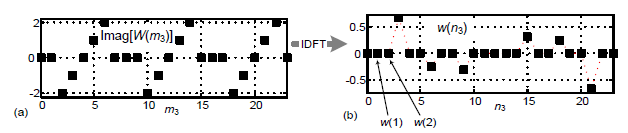
Figure 3
To compute the w(n3) time samples we perform a 24-point inverse DFT of Imag[W(m3)] using
$$w(n_3) = \frac 1{24} \cdot \sum_0^{23} Imag[W(m_3)]e^{j2\pi n_3m_3/24}\tag{1}$$
To compute Figure 3(b)'s w(1) time sample (the second sample in the sequence), we modify Eq. (1) by setting n3 = 1 as:
$$w(1) = \frac 1{24} \cdot \sum_0^{23} Imag[W(m_3)]e^{j2\pi m_3/24}\tag{2}$$
As such the real part of w(1), Real[w(1)], is:
$$Real[w(1)] = \frac 1{24} \cdot \sum_0^{23} Imag[W(m_3)] \cdot cos(2\pi m_3/24)\tag{3}$$
Pictorially, the summation in Eq. (3) is the summation of the products of the black square dots times the blue circular dots as shown in Figure 4(a). While not immediately obvious, the sum of those products is equal to zero. We show this zero-valued summation in Figure 4(b) where the black squares that produce individual zero-valued products are omitted for clarity.
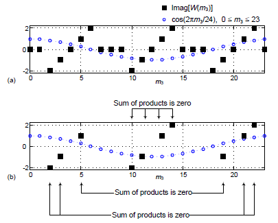
Figure 4
The imaginary part of Eq. (2)'s w(1), Imag[w(1)], is:
$$Imag[w(1)] = \frac 1{24} \cdot \sum_0^{23} Imag[W(m_3)] \cdot sin(2\pi m_3/24)\tag{4}$$
Graphically, the summation in Eq. (4) is the summation of the products of the black square dots times the blue circular dots as shown in Figure 5(a). We show Eq. (4)'s zero-valued summation in Figure 5(b) where the zero-valued black squares are omitted for clarity. The numbers on the arrows in Figure 5(b) are the individual products of square and circular sample pairs.
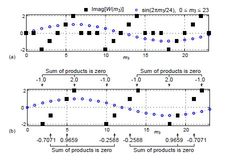
Figure 5
So, we have shown that w(1)'s real and imaginary parts are both zero-valued and now we see why w(1) = 0 in Figure 3(b).
Next, as promised, we show that Figure 3(b)'s w(2)time sample is zero-valued. To compute Figure 3(b)'s w(2)time sample, we modify Eq. (1) by setting n3 = 2 as:
$$w(2) = \frac 1{24} \cdot \sum_0^{23} Imag[W(m_3)]e^{j2\pi 2m_3/24} \tag{5}$$
$$\qquad \qquad \qquad = \frac 1{24} \cdot \sum_0^{23} Imag[W(m_3)] \cdot cos(2\pi 2m_3/24) \\ \qquad \qquad \qquad \qquad \qquad + \frac 1{24} \cdot \sum_0^{23} Imag[W(m_3)] \cdot sin(2\pi 2m_3/24) \tag{6}$$
Similar to Figure 4, the first summation in Eq. (6) is the summation of the products of the black square dots times the blue circular dots as shown in Figure 6(a). The second summation in Eq. (6) is the summation of the dots given in Figure 6(b). And both summations in Eq. (6) are equal to zero as shown in the Appendix. Thus w(2)'s real and imaginary parts are both zero-valued and now we see why w(2) = 0 in Figure 3(b).
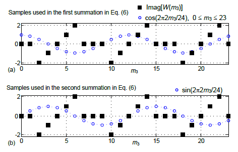
Figure 6
If we cared to do so, we could also show that the inverse DFT Figure 3's Imag[ W(m3)] sequence produces the remaining zero-valued "stuffed" samples, w(4), w(5), w(7), w(8), etc., in the w(n3) sequence. And that would, hopefully, answer this blog's question: "Why does time domain zero stuffing produce spectral replications."

Appendix
This Appendix shows why the w(2) time sample in Figure 3(b) is zero-valued.
To compute the w(2) time sample, we modify Eq. (1) by setting n3 = 2 as:
$$w(2) = \frac 1{24} \cdot \sum_0^{23} Imag[W(m_3)]e^{j2\pi 2m_3/24} \tag{A-1}$$
As such the real part of w(2), Real[w(2)], is:
$$Real[w(2)] = \frac 1{24} \cdot \sum_0^{23} Imag[W(m_3)] \cdot cos(2\pi 2m_3/24) \tag{A-2}$$
Pictorially, the summation in Eq. (A-2) is the summation of the products of the black square dots times the blue circular dots as shown in Figure A1(a). While not immediately obvious, the sum of the products is equal to zero. We show this zero-valued summation in Figure A1(b) where the zero-valued black squares are omitted for clarity.
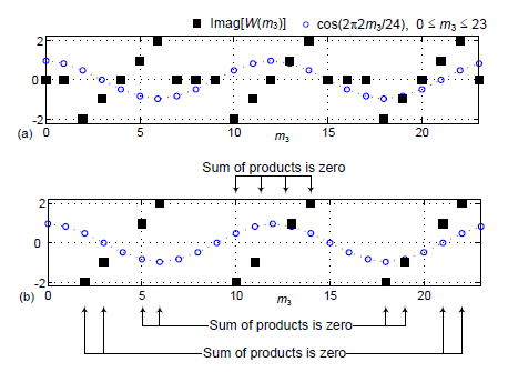
Figure A1
The imaginary part of Eq. (A-1)'s w(2), Imag[w(2)], is:
$$Imag[(w(2)] = \frac 1{24} \cdot \sum_0^{23} Imag[W(m_3)] \cdot sin(2\pi 2m_3/24) \tag{A-3}$$
Graphically, the summation in Eq. (A-3) is the summation of the products of the black square dots times the blue circular dots as shown in Figure A2(a). We show Eq. (A-3)'s zero-valued summation in Figure A2(b) where the black squares that produce individual zero-valued products are omitted for clarity. The numbers on the arrows in Figure A1(b) are the individual products of square and circular sample pairs.
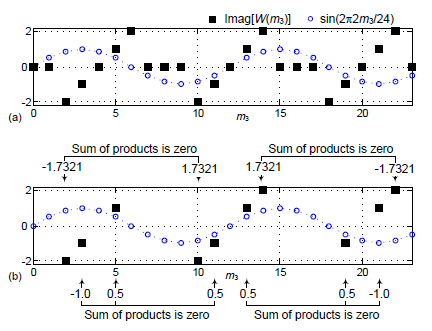
Figure A2
That concludes our proof that the Figure 3(b) w(2) time sample's real and imaginary parts are both zero-valued, thus w(2) = 0.


- Comments
- Write a Comment Select to add a comment
I was wondering what is the "z transform" of time domain zero stuffing. Could you tell me?
Am I right that the z transform of time domain zero padding is z^-m with m being the number of zeros?
Thank you in advance
پویا پاکاریان

Hi پویا پاکاریان.
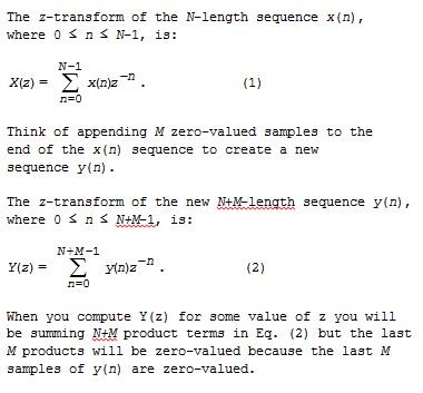
I hope that answers your question.
Many thanks Prof. Lyons
Please let me ask my question this way. Maybe this way I can explain myself better:
Suppose we have a signal named lowercase "u" whose z-transform is capital "U"
experiment 1:
Suppose we pad the signal by placing 5 zeros before it, which pushes the signal 5 steps ahead in the time domain to obtain:
lowercase "x" = [0 0 0 0 0 u]
Then we know that the z-transform of lowercase "x" will be:
X=(z^(-5)).U
with both X and U capital.
Am I right in my explanations above?
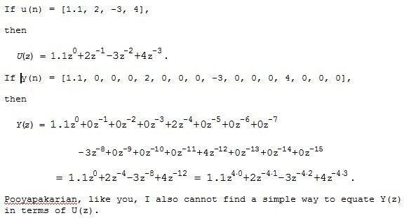
experiment 2:
Suppose we stuff our signal "u" by 3 zeros; i.e. we place 3 zeros after each single data point of it to build the signal lowercase "y". Is there a simple way to show the change that occurs in the z-transform? i.e. is there a simple relation (almost as simple as the one we saw in experiment 1 for capital "X") for capital "Y" in terms of Capital "U"?
The simplest that I can think of is in terms of lowercase "u"; as follows:
capital Y = sigma (from n=0 to N-1) of (u(n).(z^(-4n)))
with N as the length of the signal and "4" coming from the fact that we stuffed 3 zeros between any two consecutive data point of lowercase "u". (i.e. L=3 and 4=L+1)
The equation above explains capital "Y" in terms of the lowercase "u"; but I need an equation for capital"Y" in terms of capital"U" (akin to what we obtained for capital "X" in experiment 1). Does any such equation exist?
Apologies for the length of my message; and kindest regards
پویا پاکاریان
.
To post reply to a comment, click on the 'reply' button attached to each comment. To post a new comment (not a reply to a comment) check out the 'Write a Comment' tab at the top of the comments.
Please login (on the right) if you already have an account on this platform.
Otherwise, please use this form to register (free) an join one of the largest online community for Electrical/Embedded/DSP/FPGA/ML engineers:


