• Audio DSP
• Matlab
• Probability

Introduction

Last post we motivated the idea of viewing the classic phase vocoder as a Markov process. This was due to the fact that the input signal’s features are unknown to the computer, and the phase advancement for the next synthesis frame is entirely dependent on the phase advancement of the current frame. We will dive a bit deeper into this idea, and flesh out some details which we left untouched last week. This includes the effect our discrete Fourier transform has on the transition graph, different ways to interpret the correlation data, the effects which decisions we make have on the correlation data, and outlining a transition graph of our own.

Let’s remind ourselves of the purpose of this investigation: sinusoidal movement is a reality that must be dealt with when affecting the time information of a signal. However we don’t want to go so far as coding every time detail of a signal into our phase vocoder algorithm, as we would then have completely relinquished precious real-time control. Our goal then is to find some kind of middle ground between complete real-time control of an arbitrary signal, and rigid custom phase vocoders per signal. We hope to outline a transition graph which arises from thinking about the phase vocoder as a Markov chain, and which will be used to inform our phase vocoder time/frequency modification decisions. 

Properties

Let’s start by looking at the idea of a transition matrix and some of the implications of using a discrete Fourier transform. First, the size of the transition graph depends on the size of the FFT, whose frequency and time resolution are inversely proportional. So the larger the transition graph, the more time its frequency data represents. For musical signals, the longer a sinusoidal component stays in a certain frequency range, the more we should expect it to change locations. So if we consider a certain frequency range, the correlation of that frequency range to itself should be smaller the larger N we choose. This property is illustrated in the following equation.

\begin{equation}\label{eq1} N_{2} > N_{1} \Rightarrow R^{p,N_{2}}_{\omega_{1},\omega_{2}} < R^{p,N_{1}}_{\omega_{1},\omega_{2}} \end{equation}

where $R^{p}$ is the proportional correlation of a given frequency range $\omega_{1}$, with another frequency range, $\omega_{2}$, sufficiently close to $\omega_{1}$.

We can see this if we compare two proportional correlation matrices, one of size $N = 1024$ and another of size $N = 4096$. In order to properly compare these, each cell must represent the same frequency range. So we add every $4$ columns and every $4$ rows, and divide the sum by $4$ (since each row is normalized to sum to $1$ and we are adding $4$ rows.) Now we can see how the same frequency range correlates to every other frequency range for two different choices of $N$, and compare how the choice of $N$ affects this correlation. Here is the proportional correlation of a each frequency bin with itself.

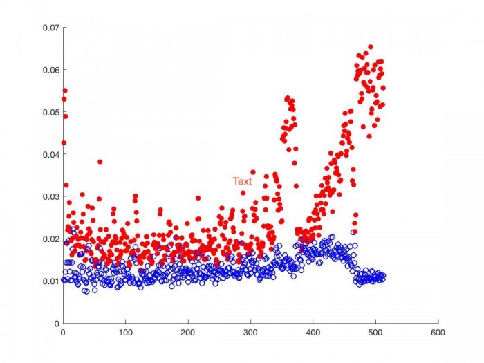
 Below we look at the proportional correlation of bin $k$ with bin $k \pm 1, k \pm 2, k \pm 3$.

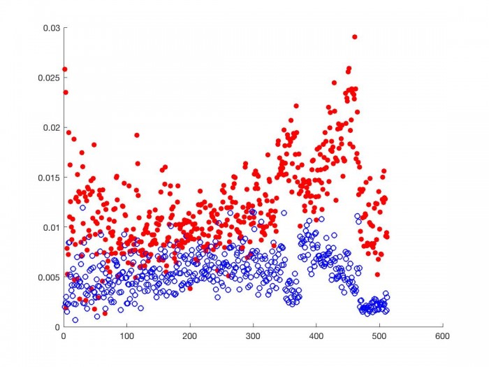
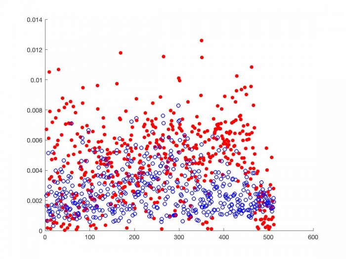
As we can see, for each frequency range, the proportional correlation matrix from the smaller N (red discs) correlates higher with frequency ranges close to it than the proportional correlation matrix from the larger N (blue circles). This is most true for frequency ranges near the one we are comparing others to, as we see above. This is the behavior we should expect given the above inequality. DSP choices regarding time affect the correlation matrix and should be considered when designing a phase vocoder transition graph.

If we think about what the phase vocoder’s main purpose is, time stretching/contracting, perhaps we should expect the time modification factor of $\alpha$  to also have some kind of effect on the correlation matrix, and consequently the transition graph. Consider the correlation matrix of a phase vocoder signal of Bach’s violin sonata in G minor [1] which has been time stretched by a factor of 2.

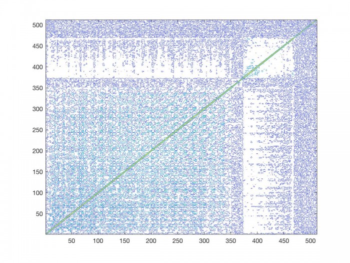
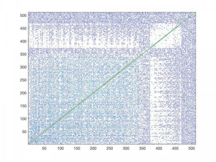
The correlation matrix of the regular signal is on the left, and half speed signal is on the right. Not surprisingly both matrices look similar. However, there are some differences that should be noted. Because we have stretched the duration of the signal by a factor of 2, any sinusoidal movement present in the signal occurs over a period of time twice as long as in the original signal. Moreover, any frequency distance traveled by a sinusoid in an analysis time period is necessarily less than in the original signal. We have now made it more likely that a given sinusoidal component will stay in the same frequency range than in the original signal. This has a similar effect on the correlation matrix as we saw above when we increased the size of the FFT. If we look at the correlation matrix of the time stretched signal, in general a given bin correlates higher with the bins closer to it than it does in the original signal. We can see this in the mean amplitude difference data, and in the amplitude difference standard deviation per frequency bin. 

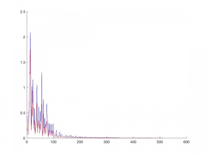
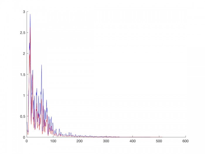
The original speed signal (blue) has a larger average amplitude difference (left) and larger amplitude difference standard deviation (right) per frequency bin than the phase vocoder signal which has been time stretched by a factor of 2 (red). Since we are interpreting amplitude difference as one of the markers of sinusoidal movement, once again this implies that the slower we are making our input signal, the more likely sinusoidal components are to stay in frequency bins close to where they currently are. Consequently, the transition graph should tend towards sinusoids staying in neighboring frequency bins.

Considerations

If we think about the features of this time stretched signal, we can start drawing conclusions about how we should construct our transition graph. We see that the slower sinusoidal movement present in the signal, the greater the correlation each bin has with the bins around it. So when we are modifying the timing of our signal by a factor of $\alpha$, our transition graph should also reflect our choice of alpha. The following equation illustrates the properties we just explored. 

\begin{equation} \label{eq2}p(x,y,\alpha) = \frac{\alpha \lceil Log_{2}(\frac{x}{64}+1)\rceil }{(x-y)^{2}}, x \neq y, \alpha > 0\end{equation}

First, we will say that the probability that a sinusoid is a given channel, $x$, will move to another given channel, $y$, is inversely proportionally to the square difference between those channels. Thus the further in the spectrum you look from a given location, the less and less likely it is as a destination. Secondly, this distance is a function of where the sinusoid is in the spectrum. The log function in the numerator creates a boundary which favors certain bins over others. Since we are using the discrete Fourier Transform, the ceiling operator is used when drawing the boundary lines. For bins who are in the boundary, the probability that they are future destinations of a given sinusoid goes up compared to the regular inverse square distance. For bins outside that boundary, the probability that they are a future destination goes down. We include the time modification factor in the numerator to contract/expand this boundary, thus mimicking the behavior we saw above. The more we slow down our signal (alpha is smaller) the smaller we draw the boundary. Conversely, the more we speed up our signal (alpha is larger) the larger we draw the boundary. The effect of larger N’s that we observed at the beginning conveniently takes care of itself. While the boundary is allowed to get larger as we choose bigger $N$'s, the frequency distance per bin is smaller the larger $N$ is. Thus our inequality from the beginning still holds true. Lastly, we have to define the probability that a given sinusoid will stay in the same place, since in the above equation, $x$ cannot equal $y$. We will let the probability that a sinusoid will stay in a given bin be one minus the average proportional amplitude change. Bins with a lower average proportional amplitude change will have a higher probability that sinusoids already occupying them will stay there. The behavior of this function is illustrated in the following graph.

When implementing this behavior in a transition graph, we will limit the scope which a sinusoid can travel. For $N = 1024$, we will consider a generous $24$ bins $\pm 1076 Hz$ for a given bin as the limit for serious destinations of a sinusoid in that location. In order to motivate this, just consider an input signal, and think about how many times a single voice jumps more than 1000 Hz: not many. Ballpark of $3$ times a minute, at most, in general. So if we assume once every $20$ seconds, that’s once every $882,000$ samples, or once every 861 FFT frames which shakes out to a probability of $.0012$ distributed over 412 bins per frame (as must be the case for a Markov process), or $.00000282$ per bin. So for now let’s just call it some small probability of $\epsilon$ and worry about more likely frequency destinations. The following transition graph in Table 1 is based on the data from the linked MATLAB code which can be found at the end of this post.

Lastly, let’s dig a bit deeper into some of the signal features we saw at the end of the previous post. It was pretty clear that the correlation matrix of an intentional signal displayed that intention, and conversely that unintentional signal’s correlation matrix displayed that lack of intention. Clearly there are more than these two categories of signals, for instance, intentional signals corrupted by noise. Let’s consider the correlation matrix for the first $7$ seconds of Bach’s violin sonata in G minor which has been corrupted with Gaussian noise. 

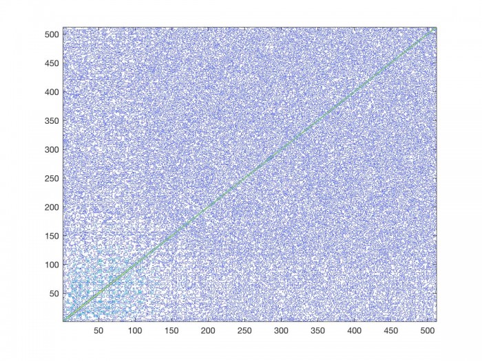
As we can see, the less clear a signal is, the less informative the correlation matrix is. Specifically the areas which showed little spectral activity have now been filled with junk. We should keep this mind as we move forward to next post. 

Conclusion

We have proposed the outline of a phase vocoder transition graph based on the correlation data from Bach's Violin Sonata in G minor. We have showed some of the effects in phase vocoder output based on choices we make. In the world of real-time audio DSP, there are few aspects that we have complete control over. So when we are presented with the fact that the decision we want to make may actually improve performance, we should take full advantage of it. This will be explored next post as we start wrapping up this investigation. 

MATLAB code

pdf download

Original Post

[1] https://www.youtube.com/watch?v=FTUWCr3IXxw

Sign in