


Convolution Representation
We will now derive the convolution representation for LTI filters
in its full generality. The first step is to express an arbitrary signal
![]() as a linear combination of shifted impulses, i.e.,
as a linear combination of shifted impulses, i.e.,
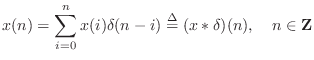
where ``
If the above equation is not obvious, here is how it is built up
intuitively. Imagine
![]() as a 1 in the midst of an
infinite string of 0s. Now think of
as a 1 in the midst of an
infinite string of 0s. Now think of
![]() as the same
pattern shifted over to the right by
as the same
pattern shifted over to the right by ![]() samples. Next multiply
samples. Next multiply
![]() by
by ![]() , which plucks out the sample
, which plucks out the sample ![]() and surrounds it on both sides by 0's. An example collection of
waveforms
and surrounds it on both sides by 0's. An example collection of
waveforms
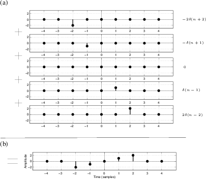
![]() for the case
for the case
![]() is shown in
Fig.5.4a. Now, sum over all
is shown in
Fig.5.4a. Now, sum over all ![]() , bringing together the
samples of
, bringing together the
samples of ![]() , to obtain
, to obtain ![]() . Figure 5.4b
shows the result of this addition for the sequences in
Fig.5.4a. Thus, any signal
. Figure 5.4b
shows the result of this addition for the sequences in
Fig.5.4a. Thus, any signal ![]() may be expressed as a
weighted sum of shifted impulses.
may be expressed as a
weighted sum of shifted impulses.
Equation (5.4) expresses a signal as a linear combination (or weighted sum) of impulses. That is, each sample may be viewed as an impulse at some amplitude and time. As we have already seen, each impulse (sample) arriving at the filter's input will cause the filter to produce an impulse response. If another impulse arrives at the filter's input before the first impulse response has died away, then the impulse response for both impulses will superimpose (add together sample by sample). More generally, since the input is a linear combination of impulses, the output is the same linear combination of impulse responses. This is a direct consequence of the superposition principle which holds for any LTI filter.
 |
We repeat this in more precise terms. First linearity is used and then
time-invariance is invoked. Using the form of the general linear
filter in Eq.![]() (4.2), and the definition of linearity,
Eq.
(4.2), and the definition of linearity,
Eq.![]() (4.3) and Eq.
(4.3) and Eq.![]() (4.5),
we can express the output of any linear (and possibly time-varying) filter by
(4.5),
we can express the output of any linear (and possibly time-varying) filter by
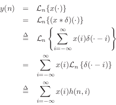
where we have written
![]() to denote the filter
response at time
to denote the filter
response at time ![]() to an impulse which occurred at time
to an impulse which occurred at time ![]() . If we are
to be completely rigorous mathematically, certain ``smoothness''
restrictions must be placed on the linear operator
. If we are
to be completely rigorous mathematically, certain ``smoothness''
restrictions must be placed on the linear operator ![]() in order that
it may be distributed inside the infinite summation [37].
However, practically useful filters of the
form of Eq.
in order that
it may be distributed inside the infinite summation [37].
However, practically useful filters of the
form of Eq.![]() (5.1) satisfy these restrictions. If in addition to
being linear, the filter is time-invariant, then
(5.1) satisfy these restrictions. If in addition to
being linear, the filter is time-invariant, then
![]() ,
which allows us to write
,
which allows us to write
This states that the filter output
The infinite sum
in Eq.![]() (5.5) can be replaced by more typical practical
limits. By choosing time 0 as the beginning of the signal, we may
define
(5.5) can be replaced by more typical practical
limits. By choosing time 0 as the beginning of the signal, we may
define ![]() to be 0 for
to be 0 for ![]() so that the lower summation limit of
so that the lower summation limit of
![]() can be replaced by 0. Also, if the filter is causal, we
have
can be replaced by 0. Also, if the filter is causal, we
have ![]() for
for ![]() , so the upper summation limit can be
written as
, so the upper summation limit can be
written as ![]() instead of
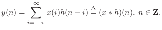
instead of ![]() . Thus, the
convolution representation of a linear, time-invariant, causal
digital filter is given by
. Thus, the
convolution representation of a linear, time-invariant, causal
digital filter is given by
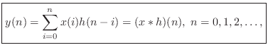
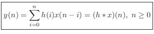
Since the above equation is a convolution, and since convolution is
commutative (i.e.,
![]() [84]), we
can rewrite it as
[84]), we
can rewrite it as
Convolution Representation Summary
We have shown that the output ![]() of any LTI filter may be calculated
by convolving the input
of any LTI filter may be calculated
by convolving the input ![]() with the impulse response
with the impulse response ![]() . It is
instructive to compare this method of filter implementation to the use
of difference equations, Eq.
. It is
instructive to compare this method of filter implementation to the use
of difference equations, Eq.![]() (5.1). If there is no feedback (no
(5.1). If there is no feedback (no
![]() coefficients in Eq.
coefficients in Eq.![]() (5.1)), then the difference equation and
the convolution formula are essentially identical, as shown in
the next section.
For recursive filters, we can convert the difference equation into a
convolution by calculating the filter impulse response. However, this
can be rather tedious, since with nonzero feedback coefficients the
impulse response generally lasts forever. Of course, for stable
filters the response is infinite only in theory; in practice, one may
truncate the response after an appropriate length of time, such as
after it falls below the quantization noise level due to round-off
error.
(5.1)), then the difference equation and
the convolution formula are essentially identical, as shown in
the next section.
For recursive filters, we can convert the difference equation into a
convolution by calculating the filter impulse response. However, this
can be rather tedious, since with nonzero feedback coefficients the
impulse response generally lasts forever. Of course, for stable
filters the response is infinite only in theory; in practice, one may
truncate the response after an appropriate length of time, such as
after it falls below the quantization noise level due to round-off
error.
Next Section:
Finite Impulse Response Digital Filters
Previous Section:
Implications of Linear-Time-Invariance


