


Example LPF Frequency Response Using freqz
Figure 7.2 lists a short matlab program illustrating usage of freqz in Octave (as found in the octave-forge package). The same code should also run in Matlab, provided the Signal Processing Toolbox is available. The lines of code not pertaining to plots are the following:
  [B,A] = ellip(4,1,20,0.5); % Design lowpass filter B(z)/A(z)
  [H,w] = freqz(B,A);        % Compute frequency response H(w)
The filter example is a recursive fourth-order elliptic function lowpass filter cutting off at half the Nyquist limit (``
  plot(w,abs(H));
  plot(w,angle(H));
However, the example of Fig.7.2 uses more detailed ``compatibility'' functions listed in Appendix J. In particular, the freqplot utility is a simple compatibility wrapper for plot with label and title support (see §J.2 for Octave and Matlab version listings), and saveplot is a trivial compatibility wrapper for the print function, which saves the current plot to a disk file (§J.3). The saved freqplot plots are shown in Fig.7.3(a) and Fig.7.3(b).8.3
[B,A] = ellip(4,1,20,0.5); % Design the lowpass filter [H,w] = freqz(B,A); % Compute its frequency response % Plot the frequency response H(w): % figure(1); freqplot(w,abs(H),'-k','Amplitude Response',... 'Frequency (rad/sample)', 'Gain'); saveplot('../eps/freqzdemo1.eps'); figure(2); freqplot(w,angle(H),'-k','Phase Response',... 'Frequency (rad/sample)', 'Phase (rad)'); saveplot('../eps/freqzdemo2.eps'); % Plot frequency response in a "multiplot" like Matlab uses: % figure(3); plotfr(H,w/(2*pi)); if exist('OCTAVE_VERSION') disp('Cannot save multiplots to disk in Octave') else saveplot('../eps/freqzdemo3.eps'); end |
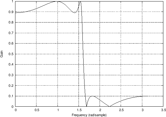
Amplitude
Response 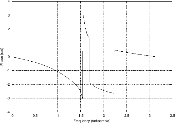
Phase Response |
Next Section:
Phase Delay
Previous Section:
Frequency Response in Matlab


