


Sampling Theory
In this appendix, sampling theory is derived as an application of the DTFT and the Fourier theorems developed in Appendix C. First, we must derive a formula for aliasing due to uniformly sampling a continuous-time signal. Next, the sampling theorem is proved. The sampling theorem provides that a properly bandlimited continuous-time signal can be sampled and reconstructed from its samples without error, in principle.
An early derivation of the sampling theorem is often cited as a 1928 paper by Harold Nyquist, and Claude Shannon is credited with reviving interest in the sampling theorem after World War II when computers became public.D.1As a result, the sampling theorem is often called ``Nyquist's sampling theorem,'' ``Shannon's sampling theorem,'' or the like. Also, the sampling rate has been called the Nyquist rate in honor of Nyquist's contributions [48]. In the author's experience, however, modern usage of the term ``Nyquist rate'' refers instead to half the sampling rate. To resolve this clash between historical and current usage, the term Nyquist limit will always mean half the sampling rate in this book series, and the term ``Nyquist rate'' will not be used at all.
Introduction to Sampling
Inside computers and modern ``digital'' synthesizers, (as well as music CDs), sound is sampled into a stream of numbers. Each sample can be thought of as a number which specifies the positionD.2of a loudspeaker at a particular instant. When sound is sampled, we call it digital audio. The sampling rate used for CDs nowadays is 44,100 samples per second. That means when you play a CD, the speakers in your stereo system are moved to a new position 44,100 times per second, or once every 23 microseconds. Controlling a speaker this fast enables it to generate any sound in the human hearing range because we cannot hear frequencies higher than around 20,000 cycles per second, and a sampling rate more than twice the highest frequency in the sound guarantees that exact reconstruction is possible from the samples.
Reconstruction from Samples--Pictorial Version
Figure D.1 shows how a sound is reconstructed from its samples. Each sample can be considered as specifying the scaling and location of a sinc function. The discrete-time signal being interpolated in the figure is a digital rectangular pulse:
![\includegraphics[width=\twidth]{eps/SincSum}](http://www.dsprelated.com/josimages_new/mdft/img1765.png) |
Notice that each sinc function passes through zero at every sample instant but the one it is centered on, where it passes through 1.
The Sinc Function
![\includegraphics[width=\twidth]{eps/Sinc}](http://www.dsprelated.com/josimages_new/mdft/img1768.png)
The sinc function, or cardinal sine function, is the famous ``sine x over x'' curve, and is illustrated in Fig.D.2. For bandlimited interpolation of discrete-time signals, the ideal interpolation kernel is proportional to the sinc function
Reconstruction from Samples--The Math
Let
![]() denote the
denote the ![]() th sample of the original
sound
th sample of the original
sound ![]() , where
, where ![]() is time in seconds. Thus,
is time in seconds. Thus, ![]() ranges over the
integers, and
ranges over the
integers, and ![]() is the sampling interval in seconds. The
sampling rate in Hertz (Hz) is just the reciprocal of the
sampling period,
i.e.,
is the sampling interval in seconds. The
sampling rate in Hertz (Hz) is just the reciprocal of the
sampling period,
i.e.,
To avoid losing any information as a result of sampling, we must
assume ![]() is bandlimited to less than half the sampling
rate. This means there can be no energy in
is bandlimited to less than half the sampling
rate. This means there can be no energy in ![]() at frequency
at frequency
![]() or above. We will prove this mathematically when we prove
the sampling theorem in §D.3 below.
or above. We will prove this mathematically when we prove
the sampling theorem in §D.3 below.
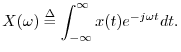
Let ![]() denote the Fourier transform of
denote the Fourier transform of ![]() , i.e.,
, i.e.,
The reconstruction of a sound from its samples can thus be interpreted as follows: convert the sample stream into a weighted impulse train, and pass that signal through an ideal lowpass filter which cuts off at half the sampling rate. These are the fundamental steps of digital to analog conversion (DAC). In practice, neither the impulses nor the lowpass filter are ideal, but they are usually close enough to ideal that one cannot hear any difference. Practical lowpass-filter design is discussed in the context of bandlimited interpolation [72].
Aliasing of Sampled Signals
This section quantifies aliasing in the general case. This result is then used in the proof of the sampling theorem in the next section.
It is well known that when a continuous-time signal contains energy at
a frequency higher than half the sampling rate ![]() , sampling
at
, sampling
at ![]() samples per second causes that energy to alias to a
lower frequency. If we write the original frequency as
samples per second causes that energy to alias to a
lower frequency. If we write the original frequency as
![]() , then the new aliased frequency is
, then the new aliased frequency is
![]() ,
for
,
for
![]() . This phenomenon is also called ``folding'',
since
. This phenomenon is also called ``folding'',
since ![]() is a ``mirror image'' of
is a ``mirror image'' of ![]() about
about ![]() . As we will
see, however, this is not a complete description of aliasing, as it
only applies to real signals. For general (complex) signals, it is
better to regard the aliasing due to sampling as a summation over all
spectral ``blocks'' of width
. As we will
see, however, this is not a complete description of aliasing, as it
only applies to real signals. For general (complex) signals, it is
better to regard the aliasing due to sampling as a summation over all
spectral ``blocks'' of width ![]() .
.
Continuous-Time Aliasing Theorem
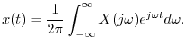
Let ![]() denote any continuous-time signal having a Fourier
Transform (FT)
denote any continuous-time signal having a Fourier
Transform (FT)
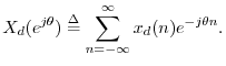
![$\displaystyle X_d(e^{j\theta}) = \frac{1}{T} \sum_{m=-\infty}^\infty X\left[j\left(\frac{\theta}{T}
+ m\frac{2\pi}{T}\right)\right].
$](http://www.dsprelated.com/josimages_new/mdft/img1788.png)
Proof:
Writing ![]() as an inverse FT gives
as an inverse FT gives
The inverse FT can be broken up into a sum of finite integrals, each of length
![]() , as follows:
, as follows:
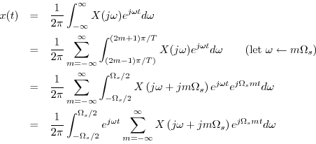
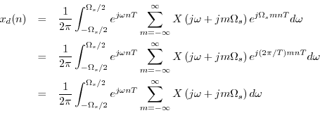
Let us now sample this representation for ![]() at
at ![]() to obtain
to obtain
![]() , and we have
, and we have
since ![]() and
and ![]() are integers.
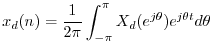
Normalizing frequency as
are integers.
Normalizing frequency as
![]() yields
yields
![$\displaystyle x_d(n) = \frac{1}{2\pi}\int_{-\pi}{\pi} e^{j\theta^\prime n}
\f...
...t(\frac{\theta^\prime }{T}
+ m\frac{2\pi}{T}\right) \right] d\theta^\prime .
$](http://www.dsprelated.com/josimages_new/mdft/img1800.png)
Sampling Theorem
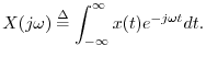
Let ![]() denote any continuous-time signal having a continuous Fourier transform
denote any continuous-time signal having a continuous Fourier transform
Proof: From the continuous-time aliasing theorem (§D.2), we
have that the discrete-time spectrum
![]() can be written in
terms of the continuous-time spectrum
can be written in
terms of the continuous-time spectrum
![]() as
as
![$\displaystyle X_d(e^{j\omega_d T}) = \frac{1}{T} \sum_{m=-\infty}^\infty X[j(\omega_d +m\Omega_s )]
$](http://www.dsprelated.com/josimages_new/mdft/img1807.png)
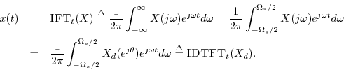
To reconstruct ![]() from its samples
from its samples ![]() , we may simply take
the inverse Fourier transform of the zero-extended DTFT, because
, we may simply take
the inverse Fourier transform of the zero-extended DTFT, because
By expanding
![]() as the DTFT of the samples
as the DTFT of the samples ![]() , the
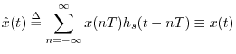
formula for reconstructing
, the
formula for reconstructing ![]() as a superposition of weighted sinc
functions is obtained (depicted in Fig.D.1):
as a superposition of weighted sinc
functions is obtained (depicted in Fig.D.1):

where we defined
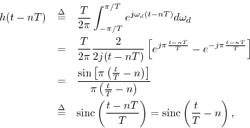
or
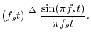
The ``sinc function'' is defined with where sinc
We have shown that when ![]() is bandlimited to less than half the
sampling rate, the IFT of the zero-extended DTFT of its samples
is bandlimited to less than half the
sampling rate, the IFT of the zero-extended DTFT of its samples
![]() gives back the original continuous-time signal
gives back the original continuous-time signal ![]() .
This completes the proof of the
sampling theorem.
.
This completes the proof of the
sampling theorem.
![]()
Conversely, if ![]() can be reconstructed from its samples
can be reconstructed from its samples
![]() , it must be true that
, it must be true that ![]() is bandlimited to
is bandlimited to
![]() , since a sampled signal only supports frequencies up
to
, since a sampled signal only supports frequencies up
to ![]() (see §D.4 below). While a real digital signal
(see §D.4 below). While a real digital signal
![]() may have energy at half the sampling rate (frequency
may have energy at half the sampling rate (frequency ![]() ),
the phase is constrained to be either 0 or
),
the phase is constrained to be either 0 or ![]() there, which is why
this frequency had to be excluded from the sampling theorem.
there, which is why
this frequency had to be excluded from the sampling theorem.
A one-line summary of the essence of the sampling-theorem proof is
The sampling theorem is easier to show when applied to sampling-rate
conversion in discrete-time, i.e., when simple downsampling of a
discrete time signal is being used to reduce the sampling rate by an
integer factor. In analogy with the continuous-time aliasing theorem
of §D.2, the downsampling theorem (§7.4.11)
states that downsampling a digital signal by an integer factor ![]() produces a digital signal whose spectrum can be calculated by
partitioning the original spectrum into
produces a digital signal whose spectrum can be calculated by
partitioning the original spectrum into ![]() equal blocks and then
summing (aliasing) those blocks. If only one of the blocks is
nonzero, then the original signal at the higher sampling rate is
exactly recoverable.
equal blocks and then
summing (aliasing) those blocks. If only one of the blocks is
nonzero, then the original signal at the higher sampling rate is
exactly recoverable.
Appendix: Frequencies Representable
by a Geometric Sequence
Consider
![]() , with
, with ![]() . Then we can write
. Then we can write
![]() in polar form as
in polar form as
Forming a geometric sequence based on ![]() yields the sequence
yields the sequence
A natural question to investigate is what frequencies ![]() are
possible. The angular step of the point
are
possible. The angular step of the point ![]() along the unit circle
in the complex plane is
along the unit circle
in the complex plane is
![]() . Since
. Since
![]() , an angular step
, an angular step
![]() is indistinguishable from
the angular step
is indistinguishable from
the angular step
![]() . Therefore, we must restrict the
angular step
. Therefore, we must restrict the
angular step ![]() to a length
to a length ![]() range in order to avoid
ambiguity.
range in order to avoid
ambiguity.
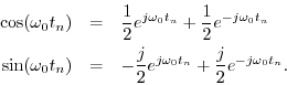
Recall from §4.3.3 that we need support for both positive and negative frequencies since equal magnitudes of each must be summed to produce real sinusoids, as indicated by the identities
The length ![]() range which is symmetric about zero is
range which is symmetric about zero is
![\begin{eqnarray*}
\omega_0 &\in& \left[-\frac{\pi}{T},\frac{\pi}{T}\right]\\
f_0&\in& \left[-\frac{f_s}{2},\frac{f_s}{2}\right].
\end{eqnarray*}](http://www.dsprelated.com/josimages_new/mdft/img1833.png)
However, there is a problem with the point at
![]() : Both
: Both
![]() and
and ![]() correspond to the same point
correspond to the same point ![]() in the
in the
![]() -plane. Technically, this can be viewed as aliasing of the
frequency
-plane. Technically, this can be viewed as aliasing of the
frequency ![]() on top of
on top of ![]() , or vice versa. The practical
impact is that it is not possible in general to reconstruct a sinusoid
from its samples at this frequency. For an obvious example, consider
the sinusoid at half the sampling-rate sampled on its zero-crossings:
, or vice versa. The practical
impact is that it is not possible in general to reconstruct a sinusoid
from its samples at this frequency. For an obvious example, consider
the sinusoid at half the sampling-rate sampled on its zero-crossings:
![]() . We cannot be expected to
reconstruct a nonzero signal from a sequence of zeros! For the signal
. We cannot be expected to
reconstruct a nonzero signal from a sequence of zeros! For the signal
![]() , on the other hand, we sample
the positive and negative peaks, and everything looks fine. In
general, we either do not know the amplitude, or we do not know phase
of a sinusoid sampled at exactly twice its frequency, and if we hit the
zero crossings, we lose it altogether.
, on the other hand, we sample
the positive and negative peaks, and everything looks fine. In
general, we either do not know the amplitude, or we do not know phase
of a sinusoid sampled at exactly twice its frequency, and if we hit the
zero crossings, we lose it altogether.
In view of the foregoing, we may define the valid range of ``digital frequencies'' to be
While one might have expected the open interval
![]() , we are
free to give the point
, we are
free to give the point ![]() either the largest positive or largest
negative representable frequency. Here, we chose the largest negative
frequency since it corresponds to the assignment of numbers in two's
complement arithmetic, which is often used to implement phase
registers in sinusoidal oscillators. Since there is no corresponding
positive-frequency component, samples at
either the largest positive or largest
negative representable frequency. Here, we chose the largest negative
frequency since it corresponds to the assignment of numbers in two's
complement arithmetic, which is often used to implement phase
registers in sinusoidal oscillators. Since there is no corresponding
positive-frequency component, samples at ![]() must be interpreted
as samples of clockwise circular motion around the unit circle at two
points per revolution. Such signals appear as an
alternating sequence of the form
must be interpreted
as samples of clockwise circular motion around the unit circle at two
points per revolution. Such signals appear as an
alternating sequence of the form
![]() , where
, where ![]() can be complex. The amplitude at
can be complex. The amplitude at ![]() is
then defined as
is
then defined as ![]() , and the phase is
, and the phase is ![]() .
.
We have seen that uniformly spaced samples can represent frequencies
![]() only in the range
only in the range
![]() , where
, where ![]() denotes the
sampling rate. Frequencies outside this range yield sampled sinusoids
indistinguishable from frequencies inside the range.
denotes the
sampling rate. Frequencies outside this range yield sampled sinusoids
indistinguishable from frequencies inside the range.
Suppose we henceforth agree to sample at higher than twice the
highest frequency in our continuous-time signal. This is normally
ensured in practice by lowpass-filtering the input signal to remove
all signal energy at ![]() and above. Such a filter is called an
anti-aliasing filter, and it is a standard first stage in an
Analog-to-Digital (A/D) Converter (ADC). Nowadays, ADCs are normally
implemented within a single integrated circuit chip, such as a CODEC
(for ``coder/decoder'') or ``multimedia chip''.
and above. Such a filter is called an
anti-aliasing filter, and it is a standard first stage in an
Analog-to-Digital (A/D) Converter (ADC). Nowadays, ADCs are normally
implemented within a single integrated circuit chip, such as a CODEC
(for ``coder/decoder'') or ``multimedia chip''.
Next Section:
Taylor Series Expansions
Previous Section:
Selected Continuous-Time Fourier Theorems


