


Off Topic: Refraction in a Varying Medium
Introduction
This article is another digression from a better understanding of the DFT. In fact, it is a digression from DSP altogether. However, since many of the readers here are Electrical Engineers and other folks who are very scientifically minded, I hope this article is of interest. A differential vector equation is derived for the trajectory of a point particle in a field of varying index of refraction. This applies to light, of course, but since it is a purely theoretical treatment it can apply to other phenomenon as well, including signal transmission.
Backstory
About five years ago, I derived an equation for describing the trajectory of a photon in a continuously varying refractive media using Snell's Law and the definition of a derivative. This article provides a different derivation resulting in the same result (18). This article is the result of how I learned to use the Euler-Lagrange equation for path optimization.
Simplifying Assumptions
The photon is considered to be a point particle. The particle is assumed to exist in a potential field where the speed of the particle at any given location is a function of the potential at that location. The second big assumption is that the potential field is static, not varying with time. There is no consideration given to energy conservation, momentum conservation, curved spacetime, dilated local time, etc. This is a purely mathematical treatment with idealized conditions. Having an equation that relates the speed to the potential is all that is required to derive a vector differential equation which describes any possible trajectory of the particle in the field.
Index of Refraction
The index of refraction $n$ is the attribute of a material that determines how fast light can pass through it. It is material and light frequency dependent. When light passes through the interface of two materials, with different indices of refraction, it appears to bend at the interface and change direction. The angles involved are related by Snell's law. This is not an article about Snell's law. What is important is the formula for the speed of light in a given material is: $$ \| \vec v \| = \frac{c}{n} = ( \vec v \cdot \vec v )^{1/2} \tag {1} $$ Where $c$ is the speed of light in a vacuum ($n=1$). Snell's Law can be derived directly from this formula. You can find that elsewhere. What is of interest here is how does the light bend when travelling through a material with a continuously varying index of refraction.
Euler-Lagrange in Refraction
The Euler-Lagrange equation is part of the field of Calculus of Variations. The goal is to find some optimized path, or trajectory, under the contraint of some condition or conditions. The standard form of the equation uses the variable $q$ to denote the path. Thus: $$ q = \vec p \tag {2} $$ The dot notation is used to indicate differentiation with respect to time. Velocity, which is a vector, is the first derivative of position. $$ \dot q = \vec v \tag {3} $$ Acceleration is the second derivative of position. It is also the first derivate of velocity. $$ \ddot q = \dot{\vec v} \tag {4} $$ The value to be optimized is set up like this: $$ T = \int_{A}^{B} F(t,q,\dot q) dt \tag {5} $$ Notice the $dt$ is not a $ds$. In this case, the optimization desired is the path with the shortest time, not the shortest distance. $T$ is the total time.
The condition that has to be met at every point on the optimal path is: $$ \frac{\partial F}{\partial q}-\frac{d}{dt}\frac{\partial F}{\partial \dot q} = 0 \tag {6} $$ $F$ needs to be set up to properly reflect the condition being met. In this case, the speed (magnitude of velocity) is defined by the value of the potential function. $F$ has to equal one because we are adding up time intervals to get the total time. The trick is to separate the one into a quotient of the the speed with itself. The velocity in the denominator is defined by the condition (1), and the speed in the numerator is kept as the magnitude of $\dot q$. $$ F = 1 = \frac{\|\dot q\|}{\|\dot q\|} = \frac{n(q)}{c} \|\dot q\| = \frac{n(q)}{c} ( \dot q \cdot \dot q )^{1/2} \tag {7} $$ Once $F$ is set up, it needs to be differentiated to fit the Euler-Lagrange optimization criteria. The speed definition is used to simplify the process. $$ \frac{\partial F}{\partial q} = \frac{\nabla n}{c} \|\dot q\| = \frac{\nabla n}{n} \tag {8} $$ $$ \begin{aligned} \frac{\partial F}{\partial \dot q} &= \frac{n}{c} \cdot \frac{1}{2} ( \dot q \cdot \dot q )^{-1/2}( 2 \dot q ) \\ &= \frac{n}{c} \cdot \frac{\dot q}{(\dot q \cdot \dot q )^{1/2} } \\ &= \frac{n^2}{c^2} \dot q \end{aligned} \tag {9} $$ The chain rule applies when calculating how the index of refraction changes in time with respect to the particle's travel. $$ \frac{dn}{dt} = \frac{dn}{dq} \cdot \frac{dq}{dt} = \nabla n \cdot \dot q \tag {10} $$ $$ \begin{aligned} \frac{d}{dt}\frac{\partial F}{\partial \dot q} &= \frac{2 n \nabla n \dot q}{c^2} \dot q + \frac{n^2}{c^2} \ddot q \\ &= \frac{1}{\dot q \cdot \dot q} \left[ 2 \left( \frac{\nabla n}{n} \cdot \dot q \right) \dot q + \ddot q \right] \end{aligned} \tag {11} $$ The differential values can now be plugged into the criteria(6). $$ \frac{\nabla n}{n} - \frac{1}{\dot q \cdot \dot q} \left[ 2 \left( \frac{\nabla n}{n} \cdot \dot q \right) \dot q + \ddot q \right] = 0 \tag {12} $$ Finally, the acceleration can be solved for yielding this differential equation. $$ \ddot q = (\dot q \cdot \dot q) \frac{\nabla n}{n} - 2 \left( \frac{\nabla n}{n} \cdot \dot q \right) \dot q \tag {13} $$
Fluff Density
The index of refraction in empty space is one. Putting it on a log scale, which makes the value zero for empty space, makes it more intuitive. $$ \rho = \ln(n) = \ln \left( \frac{ c }{ \| \vec v \| } \right) = -\ln \left( \frac{ \| \vec v \| }{ c } \right) \tag {14} $$ The value of $\rho$ can be thought of as, for lack of a better word, "fluff" density, that slows the particle down. The denser the fluff, the slower the particle can go. When there is no fluff, the particle travels at its max speed $c$.
The index of refraction value can be recovered from any fluff density value by using the exponentiation function. $$ n = e^{\rho} = \frac{c}{\| \vec v \|} \tag {15} $$ This also leads to a new speed formula based on the fluff density. $$ \| \vec v \| = c e^{-\rho} \tag {16} $$ The gradient of the fluff density can be calculated directly from (14). $$ \vec{\nabla} \rho = \frac{\nabla n}{n} \tag {17} $$
Trajectory Differential Equation
Substituting (17), (3), and (4) into (13) results in this differential vector equation: $$ \dot{\vec v} = \left( \vec v \cdot \vec v \right) \vec{\nabla} \rho - 2 \left( \vec{\nabla} \rho \cdot \vec v \right) \vec v \tag {18} $$ It is also derived directly, and simpler, in Appendix I using (16).
This equation deserves some explaining. It says that the acceleration, how its velocity is changing with time, is a linear combination of the gradient of the fluff density and the velocity. This means the acceleration always occurs in the same plane as the gradient and velocity. If the velocity is in the same line as the gradient then so is the acceleration and the equation degenerates into a solvable scalar one.
To understand what the equation means it might be better to think of a different example to which it conceptually applies. Suppose you have a truck driving through a mud field which never uses its steering. The depth of the mud corresponds to the fluff density. If there is no mud, the truck can run at full speed. If it is going through an area where the mud stays the same depth, then the gradient is zero and the truck doesn't speed up or slow down. If the truck is heading into thicker mud, then it is following the gradient and the acceleration is in the opposite direction so it is slowing down. If it is heading out of thicker mud, the it speeds up. If the truck is heading along a line of equal thickness where the mud is thicker to the right, the truck will be pulled to the right. Go ahead, go find a mud field and try it yourself.
Magnitude of the Acceleration
One of the ways you can tell when you are onto something in mathematics is when terms cancel each other out during a calculation. Calculating the magnitude of the acceleration is a fine example of this. $$ \begin{aligned} \| \dot{\vec v} \| &= \left[ \dot{\vec v} \cdot \dot{\vec v} \right]^{1/2} \\ &= \left[ \left( \left( \vec v \cdot \vec v \right) \vec{\nabla} \rho - 2 \left( \vec{\nabla} \rho \cdot \vec v \right) \vec v \right) \cdot \left( \left( \vec v \cdot \vec v \right) \vec{\nabla} \rho - 2 \left( \vec{\nabla} \rho \cdot \vec v \right) \vec v \right) \right]^{1/2} \\ &= \left[ \left( \vec v \cdot \vec v \right)^2 \vec{\nabla} \rho \cdot \vec{\nabla} \rho - 4 \left( \vec v \cdot \vec v \right) \left( \vec{\nabla} \rho \cdot \vec v \right) \vec{\nabla} \rho \cdot \vec v + 4 \left( \vec{\nabla} \rho \cdot \vec v \right)^2 \vec v \cdot \vec v \right]^{1/2} \\ &= \left[ \left( \vec v \cdot \vec v \right)^2 \vec{\nabla} \rho \cdot \vec{\nabla} \rho \right]^{1/2} \\ &= \left( \vec v \cdot \vec v \right) \| \vec{\nabla} \rho \| \\ &= \| \vec{\nabla} \rho \| \cdot \| \vec v \| ^ 2 \\ &= c^2 \| \vec{\nabla} \rho \| e^{-2\rho} \end{aligned} \tag {19} $$ The result is remarkably simple. The last line also shows that the magnitude of the acceleration is strictly a function of the value of the potential field and the gradient at that point. Of course the speed is also determined by the potential value, but the fact that the magnitude of the acceleration is the same independent of travel direction is very interesting.
Superposition of Accelerations
As a consequence of the acceleration being linear with the gradient of the potential, and the gradient operator being linear, the principle of superposition holds for the differential equation (18). In other words, if the potential field is the sum of many fields, the solution is the sum of the individual solutions. That means you can either sum the potentials first, or solve the individual fields and sum the solutions.
Here is the proof: $$ \rho = \sum_{k} \rho_k \tag {20} $$ $$ \vec{\nabla} \rho = \sum_{k} \vec{\nabla} \rho_k \tag {21} $$ $$ \begin{aligned} \dot{\vec v} &= \left( \vec v \cdot \vec v \right) \sum_{k} \vec{\nabla} \rho_k - 2 \left( \sum_{k} \vec{\nabla} \rho_k \cdot \vec v \right) \vec v \\ &= \sum_{k} \left[ \left( \vec v \cdot \vec v \right) \vec{\nabla} \rho_k - 2 \left( \vec{\nabla} \rho_k \cdot \vec v \right) \vec v \right] \\ &= \sum_{k} \dot{\vec v}_k \end{aligned} \tag {22} $$
Sideways Acceleration
The differential equation (18) can also be partitioned into a different summation of two orthogonal vector. The one vector is still in the direction of the velocity and the vector in brackets is orthogonal to the velocity or zero. $$ \dot{\vec v} = \left[ \left( \vec v \cdot \vec v \right) \vec{\nabla} \rho - \left( \vec{\nabla} \rho \cdot \vec v \right) \vec v \right] - \left( \vec{\nabla} \rho \cdot \vec v \right) \vec v \tag {23} $$ It is obvious from inspection that if the velocity is in line with the gradient then the orthogonal vector is zero lengthed. If they are not in line, then the orthogonal vector has some length. Proving it is orthogonal can be done with a simple dot product with the velocity vector. $$ \left[ \left( \vec v \cdot \vec v \right) \vec{\nabla} \rho - \left( \vec{\nabla} \rho \cdot \vec v \right) \vec v \right] \cdot \vec v = 0 \tag {24} $$ This also means the second vector, the one in the velocity direction, represents the acceleration along the velocity. In other words, how much the particle is speeding up or slowing down.
Finding the Fluff Gradient
The differential equation (18) is also invertible in a sense. The gradient vector can be found if the velocity and acceleration are known. These will be known if the trajectory is known. Here is the math:
First dot both sides of (18) with $\vec v $. $$ \dot{\vec v} \cdot \vec v = - \left( \vec{\nabla} \rho \cdot \vec v \right) \vec v \cdot \vec v \tag {25} $$ $$ \vec{\nabla} \rho \cdot \vec v = - \frac{ \dot{\vec v} \cdot \vec v }{\vec v \cdot \vec v } \tag {26} $$ Next, the value of $\vec{\nabla} \rho $ can also be solved for from (18). $$ \begin{aligned} \vec{\nabla} \rho &= \frac{ \dot{\vec v} + 2 \left( \vec{\nabla} \rho \cdot \vec v \right) \vec v }{ \vec v \cdot \vec v }\\ &= \frac{ \dot{\vec v} - 2 \left( \frac{ \dot{\vec v} \cdot \vec v }{\vec v \cdot \vec v } \right) \vec v }{ \vec v \cdot \vec v }\\ &= \frac{ \left( \vec v \cdot \vec v \right) \dot{\vec v} - 2 \left( \dot{\vec v} \cdot \vec v \right) \vec v }{ \left( \vec v \cdot \vec v \right)^2 } \end{aligned} \tag {27} $$ What's really interesting is that numerator of the final result has the same form as the differential equation, simply with the gradient and acceleration changing places.
Curvature of the Trajectory
There is a well known metric for the curvature of a trajectory. It is based on the velocity and the acceleration. It measures how much the path is bending. If the value is zero, the path is straight. Other values are always positive and represent the recipricol of the radius of a circle that matches the arc of the curve at that point.
The formula requires the cross product (there is another version for other than 3D) of the acceleration and the velocity. The angle between the two is $\theta$. $$ \begin{aligned} \kappa &= \frac{ \| \dot{\vec v} \times \vec v \|}{ \| \vec v \|^3 } \\ &= \frac{ \| \dot{\vec v} \| \cdot \| \vec v \| \sin(\theta) }{ \| \vec v \|^3 } \\ &= \frac{ \| \vec{\nabla} \rho \| \cdot \| \vec v \| ^ 2 \sin(\theta) }{ \| \vec v \|^2 } \\ &= \| \vec{\nabla} \rho \| \sin(\theta) \end{aligned} \tag {28} $$ Just like the other formulas derived from (18), this one is remarkably simple.
Stoppage Radius for a Point Source
A point source model is a classic in physics. It can be applied here as well. Assume there is a "fluff singularity", a point source where the fluff density is infinitely large, and that it falls off with the distance from the point. Thus the potential field has level surfaces that are concentric spheres around the point. The potential field is then described by a simple equation. $$ \rho = \frac{k}{r} \tag {29} $$ $k$ is just a constant that parameterizes the strength of the potential field. Since the speed of a particle in a trajectory is strictly a function of the potential function (16), the equation for the speed becomes: $$ \| \vec{ v }(r) \| = c e^{-k/r} \tag {30} $$ What is clear from this equation is that the speed is never zero. However, as the particle gets closer and closer to the center point, the density gets thicker and the particle gets slower. If the particle could reach the center, the speed would be zero. The proper way to say this mathematically is like this: $$ \lim_{r \to 0 } \| \vec{ v }(r) \| = 0 \tag {31} $$ From that, it can be said that the stoppage radius is zero which means the center point is the limit. $$ r_0 = 0 \tag {32} $$
Capture Radius for a Point Source
Sticking with the same point source model. The gradient for the potential function can also be determined. $$ \vec{\nabla} \rho = -\frac{k}{r^2} \frac{d \vec r}{\|d \vec r\|} \tag {33} $$ Notice that its strength varies with the inverse square of the distance. This is typical of point source fields. The reason is the surface area of the level surfaces, the spheres, are increasing with square of the distance. This means the quantity of whatever it is stays constant for each surface.
For any particle travelling along the sphere the acceleration will be perpendicular to the velocity. The velocity will be tangent to the sphere and the acceleration will point at the center point. The value of the $\sin \theta$ in the curvature formula (28) will be one. $$ \kappa = \| \vec{\nabla} \rho \| \cdot 1 = \frac{k}{r^2} \tag {34} $$ There is a radius value $r_*$ in which a particle travelling along a level surface sphere will form a circular orbit. This happens when the radius the point is at exactly matches the radius of curvature of the trajectory. $$ r_* = \frac{1}{\kappa} = \frac{r_*^2}{k} \tag {35} $$ Solving for the radius value gives another remarkably simple formula. If the radius of curvature is greater than the radius, the particle will escape the orbit and the point source. if the radius is closer, the particle will be captured and begin a downward spiral orbit towards the center. $$ r_* = k \tag {36} $$ The radius is proportional to the strength of the potential field. For a particle travelling this orbit, the speed can be calculated using the speed formula (34). $$ \| \vec{ v }(r_*) \| = c e^{-k/k} = c e^{-1} = \frac{c}{e} \tag {37} $$ No matter what the potential field strength around a point source is, the speed a particle in an orbit at the capture radius is always the same.
Speculations
My original intent was to compare the behavior of light in a refractive media versus the effects of light slowing down due to being in a gravity field. I made a considerable amount of progress showing they were very similar and then I found out that I had an incomplete equation governing the speed of light in gravity. It is still my goal to find, if it exists, a differential vector equation for light bending around a star (or anywhere) with the accleration as a function of the gravity gradient and the velocity.
Conclusion
The equivalent of Snell's Law was derived for refraction in a medium with a varying index of refraction demonstrating the use of the Euler-Lagrange optimization technique. As far as I know, these formulas are novel. Extensive searching on my part has not found them anywhere else. The great number of simplifications that spontaneously occur during the derivations indicates that the math has fundamental significance. I am hoping that the readers of this blog have found it interesting, and even more that someone may find a direct application in a signal processing context.
Appendix I: Euler-Lagrange in Fluff
The Euler-Lagrange method works just as well using the fluff density definition instead of the index of refraction. Using (16) for the speed, the opimizatoin function becomes: $$ F = 1 = \frac{\|\dot q\|}{\|\dot q\|} = \frac{1}{ce^{-\rho}} \|\dot q\| = \frac{e^{\rho}}{c} ( \dot q \cdot \dot q )^{1/2} \tag {38} $$ From here the process is the same. $$ \frac{\partial F}{\partial q} = \frac{e^{\rho} \nabla \rho}{c} \|\dot q\| = \nabla \rho \tag {39} $$ $$ \begin{aligned} \frac{\partial F}{\partial \dot q} &= \frac{e^{\rho}}{c} \cdot \frac{1}{2} ( \dot q \cdot \dot q )^{-1/2}( 2 \dot q ) \\ &= \frac{e^{\rho}}{c} \cdot \frac{\dot q}{(\dot q \cdot \dot q )^{1/2} } \\ &= \frac{e^{2\rho}}{c^2} \dot q \end{aligned} \tag {40} $$ $$ \frac{d\rho}{dt} = \frac{d\rho}{dq} \cdot \frac{dq}{dt} = \nabla \rho \cdot \dot q \tag {41} $$ $$ \begin{aligned} \frac{d}{dt}\frac{\partial F}{\partial \dot q} &= \frac{2 e^{2\rho} \nabla \rho \dot q}{c^2} \dot q + \frac{e^{2\rho}}{c^2} \ddot q \\ &= \frac{e^{2\rho}}{c^2} \left[ 2 \left( \nabla \rho \cdot \dot q \right) \dot q + \ddot q \right] \end{aligned} \tag {42} $$ $$ \nabla \rho - \frac{e^{2\rho}}{c^2} \left[ 2 \left( \nabla \rho \cdot \dot q \right) \dot q + \ddot q \right] = 0 \tag {43} $$ $$ (\dot q \cdot \dot q) \nabla \rho - \left[ 2 \left( \nabla \rho \cdot \dot q \right) \dot q + \ddot q \right] = 0 \tag {44} $$ $$ \ddot q = (\dot q \cdot \dot q) \nabla \rho - 2 \left( \nabla \rho \cdot \dot q \right) \dot q \tag {45} $$ Finally, the $q$ based terms can be expressed as the velocity vectors instead. $$ \dot{\vec v} = \left( \vec v \cdot \vec v \right) \vec{\nabla} \rho - 2 \left( \vec{\nabla} \rho \cdot \vec v \right) \vec v \tag {46} $$ The result is the same remarkable differential vector equation.


- Comments
- Write a Comment Select to add a comment

I have found yet another derivation of this formula using what is known as the eikonal equation.
Here is the eikonal equation with the chain rule applied, value substitution, and applying \(|v|=c/n\).
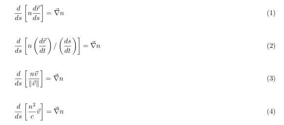
Then the derivative is taken and the derivative values inside the brackets are resolved.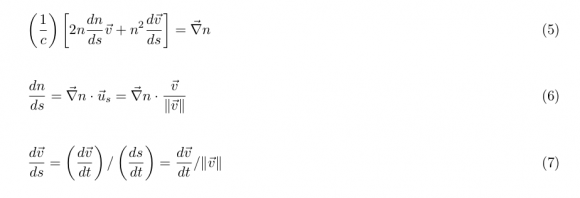
Substitute them in and multiply both sides by \(|v|\), and then again, \(|v| = c/n\).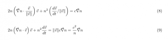
Solve for the acceleration as a linear combination of the gradient and the velocity, and finally substitute v*v back in for \(c^2/n^2\).
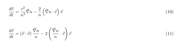
There you have it. The vector differential form of the eikonal equation.
To post reply to a comment, click on the 'reply' button attached to each comment. To post a new comment (not a reply to a comment) check out the 'Write a Comment' tab at the top of the comments.
Please login (on the right) if you already have an account on this platform.
Otherwise, please use this form to register (free) an join one of the largest online community for Electrical/Embedded/DSP/FPGA/ML engineers:


