I just learned a new method (new to me at least) for computing the group delay of digital filters. In the event this process turns out to be interesting to my readers, this blog describes the method. Let's start with a bit of algebra so that you'll know I'm not making all of this up.

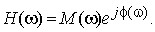
Assume we have the N-sample h(n) impulse response of a digital filter, with n being our time-domain index, and that we represent the filter's discrete-time Fourier transform (DTFT), H(ω), in polar form as:

      (1)

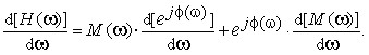
In Eq. (1), M(ω) is the frequency magnitude response of the filter, Φ(ω) is the filter's phase response, and ω is continuous frequency measured in radians/second. Taking the derivative of H(ω) with respect to ω, we have:

      (2)

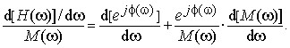
Dividing Eq. (2) by M(ω), we write:

      (3)

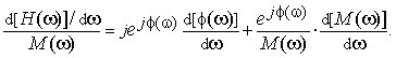
Performing the derivative of the first term on the right side of Eq. (3) gives us:

      (4)

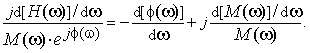      (5)

So now what does that puzzling gibberish in Eq. (5) tell us? As it turns out, it tells us a lot if we recall the following items:

• jd[H(ω)]/dω = the DTFT of n·h(n)
• M(ω)•e^jΦ(ω) = H(ω) = the DTFT of h(n)
• –d[Φ(ω)]/dω = group delay of the filter.

Now we are able to translate Eq. (5) into the meaningful expression

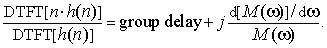      (6)

Discretizing expression (6) by replacing the DTFT with the discrete Fourier transform (DFT), we arrive at what I recently learned about computing the group delay of a digital filter:

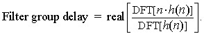      (7)

So, starting with a filter's N-sample h(n) impulse response, performing two N-point DFT's and an N-sample complex division, we can compute the filter's group delay measured in samples. (Of course, to improve our group delay granularity we can zero pad our original h(n) before computing the DFTs). The advantage of the process in expression (7) is that the phase unwrapping process needed in traditional group delay algorithms is not needed here.

WARNING Will Robinson: in implementing the process in expression (7) you must be prepared to accommodate the situation where a frequency-domain DFT[h(n)] sample is zero-valued.

Below is a bit of MATLAB code that can be used to demonstrate the process in expression (7).

clear, clc
Npts = 128;  % Number of plotting points

% Define filter feedforward & feedback coefficients
  B = [0.03, 0.0605, 0.121, 0.0605, 0.03]; 
  A = [1, -1.194, 0.436];  

  Imp_Resp_Length = 40;
  [Imp_Resp,n] = impz(B,A,Imp_Resp_Length);
  ImpResp_times_Time = Imp_Resp.*n;
  [Freq_Resp, W] = freqz(Imp_Resp, 1, Npts, 'whole');
  [Deriv_of_Freq_Resp, W] = freqz(ImpResp_times_Time, ...
      1, Npts, 'whole');
  
  Grp_Delay = real(Deriv_of_Freq_Resp./Freq_Resp);
  Grp_Delay = fftshift(Grp_Delay);
  Freq = (W-pi)/(2*pi);  % Freq axis vector

  figure(1), clf
  subplot(2,1,1)
  plot(n, Imp_Resp, '-ks', ...
        n, ImpResp_times_Time, '-bs', 'markersize', 4)
  legend('h(n)','n times h(n)');
  ylabel('Amplitude'), xlabel('n'), grid on, zoom on
  subplot(2,1,2)
  plot(Freq, Grp_Delay,'-rs', 'markersize', 4)
  ylabel('Group Delay (samples)')
  xlabel('Freq x Fs   (Fs = sample rate)')
  grid on, zoom on

JOS wrote:

Sasha Case wrote:

Rick Lyons wrote:

Rick Lyons wrote: