Correcting an Important Goertzel Filter Misconception

Recently I was on the Signal Processing Stack Exchange web site (a question and answer site for DSP people) and I read a posted question regarding Goertzel filters [1]. One of the subscribers posted a reply to the question by pointing interested readers to a Wikipedia web page discussing Goertzel filters [2]. I noticed the Wiki web site stated that a Goertzel filter:

"...is marginally stable and vulnerable to
numerical error accumulation when computed using
low-precision arithmetic and long input sequences."

That statement can often be misinterpreted. Because of that possible stability misconception, and the fact the literature of the Goertzel algorithm doesn't discuss Goertzel filter stability, I decided to write this blog.

This article is also available in PDF format

Goertzel Filter Descriptions
Typical DSP textbook descriptions of Goertzel filters begin by discussing the network shown in Figure 1(a) that can be used to compute N-point discrete Fourier transform (DFT) X(k) spectral samples [3]–[5].

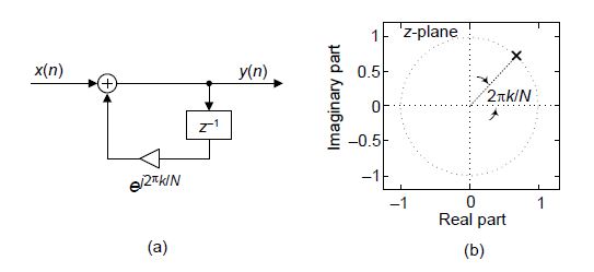
Figure 1 - Recursive network used to compute a single
DFT spectral sample: (a) implementation;
(b) z-plane pole.

The Figure 1(a) complex resonator's z-domain transfer function is

$$ H_R(z) = {1\over {1 - e^{j2 \pi k/N} z^{-1}}}\tag{1} $$

which, with infinite-precision arithmetic, has a single pole located on the z-plane's unit circle as shown in Figure 1(b).

While the Figure 1(a) resonator can be used to compute individual N-point DFT spectral samples it has a major flaw. When finite-precision arithmetic (as in our digital implementations) is used the network's z-plane pole does not lie exactly on the unit circle. This means the resonator can be unstable and a computed DFT sample value will be incorrect. In the literature of DSP the resonator is referred to as "marginally stable."

We show this in Figure 2 for various z-plane poles, in the frequency range of $ 0 \le 2\pi k/N \le \pi /2 $ radians (zero to one quarter of the input sample rate in Hz), when 5-bit binary arithmetic is used.

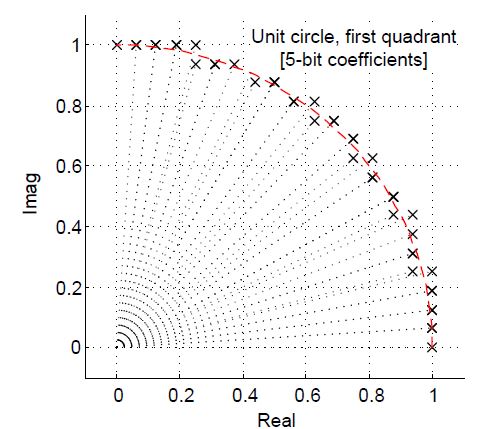
Figure 2 - First quadrant z-plane pole locations of a
complex resonator using 5-bit arithmetic.

DSP textbook descriptions of Goertzel filters don't discuss the complex resonator's unstable operation. That's because they move on to improve the computational efficiency of the complex resonator by multiplying Eq. (1)'s numerator and denominator by $ (1 - e^{-j2 \pi k/N}) $ as:

$$ H_G(z) = {1\over {1 - e^{j2 \pi k/N} z^{-1}}} \cdot {{1 - e^{-j2 \pi k/N} z^{-1}} \over  {1 - e^{-j2 \pi k/N} z^{-1}} } \tag{2}$$

$$ \qquad \qquad = {{1 - e^{-j2 \pi k/N} z^{-1}} \over {(1 - e^{j2 \pi k/N} z^{-1})(1 - e^{-j2 \pi k/N} z^{-1})}} \tag{3}$$

$$ \qquad \qquad =  {{1 - e^{-j2 \pi k/N} z^{-1}} \over {1 - 2cos(2 \pi k/N)z^{-1} + z^{-2}}} \tag{4}$$

which is the z-domain transfer function of the standard Goertzel filter. The Eq. (4) Goertzel filter's block diagram, shown in Figure in Figure 3(a), has two conjugate poles and a single pole-canceling zero on the z-plane as shown in Figure 3(b).

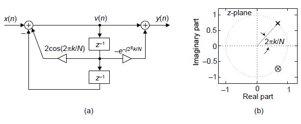
Figure 3 - Standard Goertzel filter: (a) filter
implementation; (b) z-plane poles and zero.

The Goertzel Filter Misconception
The potential misconception, regarding finite-precision arithmetic, is the following:

Misconception:
Because the first ratio in Eq. (2), which is only marginally
stable, times a unity-valued ratio equals Eq. (4), then the
implementation of Eq. (4) must also be only marginally stable.

I'm familiar with this misunderstanding because I was painfully guilty of it myself years ago -- and this is the misconception stated on the Goertzel Wikipedia web site [2].

The Stability of a Goertzel Filter
As it turns out, a Goertzel filter, described by Eq. (4), is guaranteed stable! The filter's poles always lie on the z-plane's unit circle. (Proof of that statement is given in Appendix A.)

So, we can say:

The poles of the Figure 3(a) Goertzel filter always lie
exactly on the z-plane's unit circle making the filter
guaranteed stable regardless of the numerical precision
of its coefficients.

We show this Goertzel filter stability behavior in Figure 4 for various first quadrant z-plane poles for 5-bit binary filter coefficients.

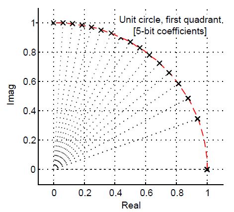
Figure 4 First quadrant z-plane pole locations of a
Goertzel filter using 5-bit arithmetic.

The Limitations of the Goertzel Filter
In finishing this blog I'll mention two important characteristics of a Goertzel filter.

[1] While the Goertzel filter is guaranteed stable, quantized coefficients (a finite number of binary bits) limit the locations where the filter's z-plane poles can be placed on the unit circle. A small number of binary bits used to represent the filter's coefficients limits the precision with which we can specify the filter's resonant frequency.

[2] Quantized coefficients make it difficult to build Goertzel filters that have low resonant frequencies. The lower the desired filter resonent frequency the larger must be the number of coefficient binary bits used.

We illustrate both of those characteristics in Figure 5 and Figure 6 for 5- and 8-bit coefficients.

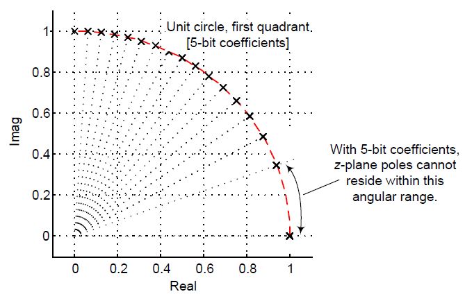
Figure 5 First quadrant z-plane pole locations of a
Goertzel filter using 5-bit arithmetic.

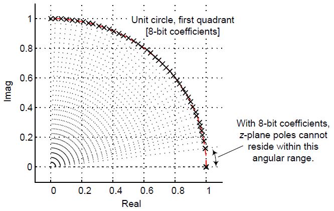
Figure 6 First quadrant z-plane pole locations of a
Goertzel filter using 8-bit arithmetic.

Conclusion
Here we showed that Goertzel filters will never be unstable due to z-domain pole placement on the z-plane's unit circle. However as pointed out by Ollie Niemitalo, another form of instability is possible with Goertzel filters. A Goertzel filter can become unstable, due to finite precision arithmetic being used for the first feedback accumulator (adder) in Figure 3 to produce the v(n) sequence, for very large values of N. So the user must take care to ensure that, for large N (in the tens of thousands for 32-bit floating point numbers), all binary register word widths can accommodate all necessary arithmetic operations. 

APPENDIX A – Proof of Goertzel Filter Guaranteed Stability
Goertzel filters, described by Eq. (4), are guaranteed stable. Proof of that statement was shown to me by the skilled DSP engineer Prof. Pavel Rajmic (Brno University of Technology, Czech Republic). Rajmic's straightforward proof of Goertzel filter stability goes like this:

For mathematical convenience, multiply the Goertzel filter's Eq. (4) numerator and denominator by $z^2$ as:

$$  {{1 - e^{-j2 \pi k/N} z^{-1}} \over {1 - 2cos(2 \pi k/N)z^{-1} + z^{-2}}} \cdot {{z^2} \over {z^2}}  $$

$$  \qquad = {{z^2 - e^{-j2 \pi k/N} z^1} \over {z^2 - 2cos(2 \pi k / N)z + 1}}\tag{A-1} $$

If we substitute $ \alpha = cos(2 \pi k/N) $ into Eq. (A-1) then Eq. (A-1)'s denominator becomes:

The roots of this polynomial will be the z-plane locations of the trtaditional Goertzel filter's poles.

The roots of the polynomial are:

Because $ \alpha $ is in the range $ -1 \le \alpha \le 1 $, then $ \alpha^2 \le 1 $ and we can rewrite expression (A-3) as:

$$  z = \alpha \pm \sqrt{-(1 - \alpha^2)} = \alpha \pm j \sqrt{1 - \alpha^2}\tag{A-4} $$

The magnitudes of both of the two complex conjugate poles are:

which is what I set out to show. So, a Goertzel filter's poles always lie exactly on the z-plane's unit circle.

References

[1] Signal Processing Stack Exchange, http://dsp.stackexchange.com/

[2] Goertzel algorithm, https://en.wikipedia.org/wiki/Goertzel_algorithm

[3] S. Mitra, "Digital Signal Processing", Fourth Edition, McGraw Hill Publishing, 2011, pp. 618-620.

[4] J. Proakis and D. Manolakis, "Digital Signal Processing-Principles, Algorithms, and Applications", Third Edition, Prentice Hall, Upper Saddle River, New Jersey, 1996, pp. 480-481.

[5] A. Oppenheim, R. Schafer, and J. Buck, "Discrete-Time Signal Processing", Second Edition, Prentice Hall, Upper Saddle River, New Jersey, 1996, pp. 633-634.

Sign in