Implementing Simultaneous Digital Differentiation, Hilbert Transformation, and Half-Band Filtering

Recently I've been thinking about digital differentiator and Hilbert transformer implementations and I've developed a processing scheme that may be of interest to the readers here on dsprelated.com.

This blog presents a novel method for simultaneously implementing a digital differentiator (DD), a Hilbert transformer (HT), and a half-band lowpass filter (HBF) using a single tapped-delay line and a single set of coefficients. The method is based on the similarities of the three N = 15-sample impulse responses shown on the left side of Figure 1. (The equations used to compute the impulse responses are given later in this blog.)

On the right side of Figure 1 we show the frequency responses of a typical DD, HT, and HBF.

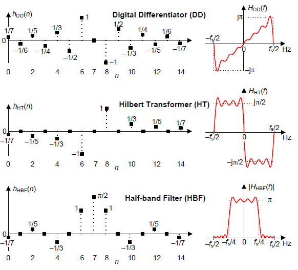
Figure 1: Impulse, and frequency, responses, of an
N = 15-point digital differentiator, Hilbert
transformer, and half-band lowpass filter.

Thinking of the above impulse response samples as tapped-delay line coefficients we see that a HBF's coefficients (with the exception of its center coefficient) and a HT's coefficients are all contained in the N-point DD's coefficients. These relationships lead us to the proposed simultaneous processing scheme shown in Figure 2 for N = 15.

The large rectangles in Figure 2 containing the $ \sum $ symbol represent arithmetic summation (an accumulator).

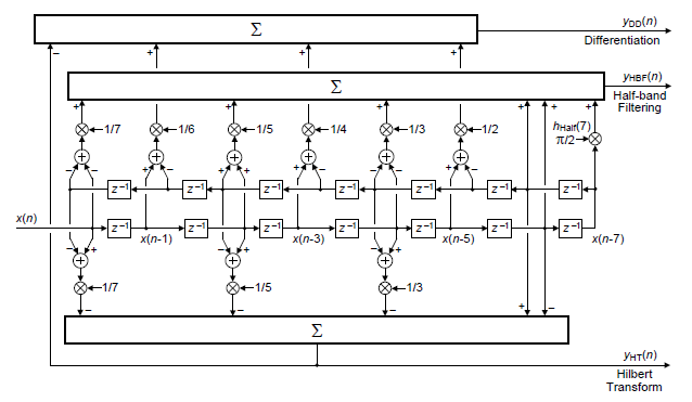
Figure 2: Simultaneous implementation of an N = 15
coefficient digital differentiator, Hilbert
transformer, and half-band lowpass filter.

The system in Figure 2 is the primary topic of this blog. If this system interests you, please read on.

When a unit sample is our input in Figure 2 the system's three impulse response outputs are those shown on the left side in Figure 1. If half-band lowpass filtering is not needed, Figure 3 shows the simultaneous implementation of a DD and a HT for N = 15.

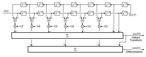
Figure 3: Simultaneous implementation of an N = 15
digital differentiator and Hilbert transformer.

Implementation Advantages

Not only do the systems in Figures 2 and 3 perform the described simultaneous processing, they do so in a surprisingly efficient manner as described in Appendix A.

Another benefit of the Figure 2 and 3 processing is that only one set of precomputed coefficients need be stored in hardware memory.

The Impulse Response Equations

The impulse response samples shown in Figure 1 (and later the coefficients in Figures 2 and 3) are obtained as follows: the coefficients of a standard N-point (N is odd) wideband DD (See references [DD_1-DD_3]) are

where M = (N-1)/2. The causal time-domain index n is 0 ≤ n ≤ N–1. In Eq. (1) when index n = M the h_DD(M) center coefficient is set to zero.

Next, if we multiply the standard textbook N-point digital HT's coefficients (See references [HT_1-HT_4]) by π/2 we obtain our scaled HT coefficients of

In Eq. (2) when index n = M the h_HT(M) center coefficient is set equal to zero. The passband gain of our Figure 2 HT process is π/2.

Finally, if we multiply the coefficients of a traditional N-point digital HBF (See references [HBF_1-HBF_3]) by π we obtain our scaled HBF coefficients of

For our Figure 2 processing, Eq. (3)'s h_HBF(M) center coefficient is set equal to π/2. The passband gain of our HBF process is π.

The Eqs. (1), (2), and (3) coefficients, for N = 15, are plotted in Figure 1. This blog's focus is strictly on odd-length h_DD(n), h_HT(n), and h_HBF(n) processing. The relationships between even-length h_DD(n), h_HT(n), and h_HBF(n) coefficients fall under the category of "For Future Study."

Passband Ripple Reduction

A nice feature of the Figures 2 and 3 systems is that any modification made to reduce the frequency-domain passband gain ripple of the Eq. (1) h_DD(n) coefficients automatically reduces the ripple in the HT's and HBF's frequency magnitude responses.

For example, the dotted red curve in Figure 4(a) shows the frequency magnitude response of the Eq. (1) DD's h_DD(n) coefficients. Multiplying h_DD(n) by a Hanning window sequence produces the reduced-ripple magnitude response shown by the solid black curve. We can see that windowing the DD's Eq. (1) coefficients reduces the HT's and the HBF's passband ripple as shown by the solid black curves in Figures 4(b) and 4(c).

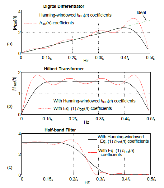
Figure 4: Frequency magnitude responses using Eq. (1)'s
h_DD(n) coefficients (dotted), and magnitude
responses after windowing Eq. (1)'s h_DD(n)
coefficients (solid).

It's also acceptable to use the Parks-McClellan, or some other, DD design method to obtain new h_DD(n) coefficients that have improved frequency-domain behavior. However, when using h_DD(n) coefficients other than those defined by Eq. (1) care must be taken to ensure that the HBF's h_HBF(M) center coefficient (the π/2 on the right side of Figure 2) be set equal to π/2 times the new differentiator's h_DD(M-1) coefficient.

Conclusion

We presented methods for performing simultaneous digital differentiation, Hilbert transformation, and half-band lowpass filtering. The methods are computationally efficient and require a minimum of coefficient storage. To borrow a slogan from the Aston Martin automobile company, the processing in Figures 2 and 3 are "engineered to exceed all expectations."

References

Differentiators:

[DD_1] R. Lyons, Understanding Digital Signal Processing, 3rd Ed., Prentice Hall, Englewood Cliffs, New Jersey, 2011, pp. 369.

[DD_2] S. Mitra, Digital Signal Processing, 4th Ed., McGraw Hill Publishing, 2011, pp. 534.

[DD_3] J. Proakis and D. Manolakis, Digital Signal Processing-Principles, Algorithms, and Applications, 3rd Ed., Prentice Hall, Upper Saddle River, New Jersey, 1996, pp. 652.

Hilbert Transformers:

[HT_1] R. Lyons, Understanding Digital Signal Processing, 3rd Ed., Prentice Hall, Englewood Cliffs, New Jersey, 2011, pp. 488.

[HT_2] S. Mitra, "Digital Signal Processing", 4th Ed., McGraw Hill Publishing, 2011, pp. 534.

[HT_3] J. Proakis and D. Manolakis, Digital Signal Processing-Principles, Algorithms, and Applications, 3rd Ed., Prentice Hall, Upper Saddle River, New Jersey, 1996, pp. 659.

[HT_4] A. Oppenheim, R. Schafer, and J. Buck, Discrete- Time Signal Processing, 2nd Ed., Prentice Hall, Englewood Cliffs, New Jersey, 1999, pp. 792.

Half-band Filters:

[HBF_1] S. Mitra, Digital Signal Processing, 4th Ed., McGraw Hill Publishing, 2011, pp. 786.

[HBF_2] F. Harris, Multirate Signal Processing for Communication Systems, Prentice-Hall, Upper Saddle River, New Jersey, 2004, pp. 203.

[HBF_3] P. Vaidyanathan, Multirate Systems and Filter Banks, Prentice Hall; Upper Saddle River, New Jersey, 1992, pp. 155.

Appendix A: Computational Efficiency

Here we describe the favorable computational efficiency of the Figures 2 and 3 systems.

For example, with symmetrical coefficients there are two traditional implementations for tapped-delay line processing. For odd N, one method uses a standard textbook inline tapped-delay line having N-1 delay elements, N multipliers, and N adders as shown in Figure A-1(a). The more computationally-efficient method uses a folded-delay line with N-1 delay elements, (N+1)/2 multipliers, and N adders as shown in Figure A-1(b).

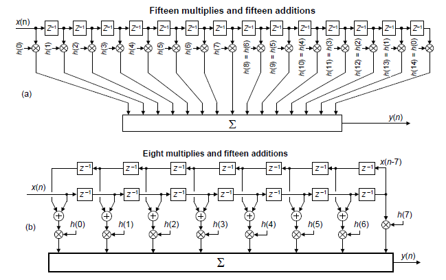
Figure A-1: Traditional tapped-delay line structures for N = 15:
(a) inline delay line method; (b) folded-delay
line method.

Fortunately, our Figures 2 and 3 systems are more computationally efficient, in terms of arithmetic operations per input sample, than either of the traditional Figure A-1 delay line implementations. Table A-1 compares the number of necessary arithmetic operations of the inline delay, folded-delay, and Figures 2 and 3 systems for N = 15.

Table A-1: Necessary Computations, Per Input Sample, For N = 15

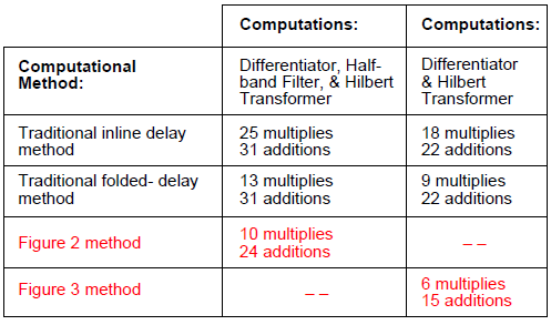
The bottom three rows of the table show us that the proposed Figure 2 and 3 systems are more computationally efficient than the popular folded-delay line processing method. And, happily, for N > 15 (a larger number of coefficients) the Figure 2 and 3 systems' computational advantages over the traditional folded-delay implementation become even more pronounced beyond that of the N = 15 case.

Sign in