


Resampling on arbitrary grid (vectorized)
Resamples a band-limited cyclic signal on an arbitrary grid via a vectorized evaluation of the Fourier series at the requested locations. The special case with signal energy at the Nyquist limit (-1, 1, -1, 1, ... component) is handled correctly.
The following two examples show resampling of two arbitrary signals:
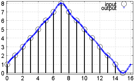
Fig. 1: Arbitrary signal example
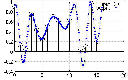
Fig. 2: Another example
The picture below illustrates the special case at the Nyquist limit:
Since the Fourier series coefficients are determined on a regular sampling grid, the outermost positive and negative frequencies are ambiguous.
The implementation provides some "interpretation" to resolve the ambiguity (using the additional constraint that a purely real-valued input signal should result in a purely real-valued output signal).
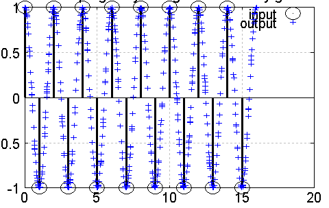
Fig. 3: Resampling a signal component at the Nyquist limit
A possible application is the generation of reference output signals for resampler design using least-mean-square methods, for example.
A related implementation that resamples on a regular grid (convert a n1-point cyclic signal to n2 samples) can be found here.
% **************************************************************
% Efficient resampling of a cyclic signal on an arbitrary grid
% M. Nentwig, 2011
% => calculates Fourier series coefficients
% => Evaluates the series on an arbitrary grid
% => takes energy exactly on the Nyquist limit into account (even-
%    size special case)
% => The required matrix calculation is vectorized, but conceptually
%    much more CPU-intensive than an IFFT reconstruction on a regular grid
% **************************************************************
close all; clear all;

% **************************************************************
% example signals
% **************************************************************
sig = [1 2 3 4 5 6 7 8 7 6 5 4 3 2 1 0];
%sig = repmat([1 -1], 1, 8); % highlights the special case at the Nyquist limit
%sig = rand(1, 16);

nIn = size(sig, 2);

% **************************************************************
% example resampling grid
% **************************************************************
evalGrid = rand(1, 500);
evalGrid = cumsum(evalGrid);
evalGrid = evalGrid / max(evalGrid) * nIn;
nOut = size(evalGrid, 2);

% **************************************************************
% determine Fourier series coefficients of signal
% **************************************************************
fCoeff = fft(sig);
nCoeff = 0;
if mod(nIn, 2) == 0
    % **************************************************************
    % special case for even-sized length: There is ambiguity, whether
    % the bin at the Nyquist limit corresponds to a positive or negative
    % frequency. Both give a -1, 1, -1, 1, ... waveform on the
    % regular sampling grid.
    % This coefficient will be treated separately. Effectively, it will
    % be interpreted as being half positive, half negative frequency.
    % **************************************************************
    bin = floor(nIn / 2) + 1;
    nCoeff = fCoeff(bin);
    fCoeff(bin) = 0; % remove it from the matrix-based evaluation
end

% **************************************************************
% indices for Fourier series
% since evaluation does not take place on a regular grid,
% one needs to distinguish between negative and positive frequencies
% **************************************************************
o = floor(nIn/2);
k = 0:nIn-1;
k = mod(k + o, nIn) - o;

% **************************************************************
% m(yi, xi) = exp(2i * pi * evalGrid(xi) * k(yi))
% each column of m evaluates the series for one requested output location
% **************************************************************
m = exp(2i * pi * transpose(repmat(transpose(evalGrid / nIn), 1, nIn) ...
                            * diag(k))) / nIn;
% each output point is the dot product between the Fourier series
% coefficients and the column in m that corresponds to the location of
% the output point
out = fCoeff * m;
out = out + nCoeff * cos(pi*evalGrid) / nIn;

% **************************************************************
% plot
% **************************************************************
out = real(out); % chop off roundoff error for plotting
figure(); grid on; hold on;
h = stem((0:nIn-1), sig, 'k'); set(h, 'lineWidth', 3);
h = plot(evalGrid, out, '+'); set(h, 'markersize', 2);
legend('input', 'output');
title('resampling of cyclic signal on arbitrary grid');


