Resampling by Lagrange-polynomial interpolation

Calculates Lagrange-resampler coefficients and resamples an example signal.

A Lagrange-resampler evaluates the unique n-th order polynomial that crosses through n+1 input samples.
This code snippet maps it to a generic Farrow structure with n+1 taps and n+1 polynomial coefficients per tap.

Fig. 1 shows the impulse response of a four-point resampler (3rd order polynomial), and a published reference result from literature, which can be found in the code.
The circles illustrate the output [0, 1, 0] from the Lagrange polynomial corresponding to the center FIR tap, when evaluated for an offset x = 0.

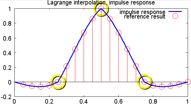
^{Fig. 1: Impulse response for four-point (cubic) Lagrange interpolation}

Fig. 2 compares the impulse responses for increasing order with the ideal sinc() response, which is aymptotically approached as the order increases:

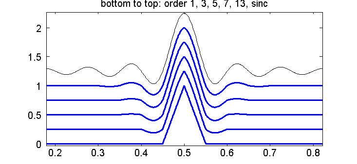
^{Fig. 2: Impulse responses for increasing interpolation order, and sinc() response.}

Copy the code snippet into lagrangeResamplingDemo.m and run it by its name in Matlab / Octave.

_{Update 18.8.2011: Fixed a bug with the final two assert() statements. Now it works in OctaveForge and Matlab.}

Update 3.8.2012: An alternative version that resamples an actual signal can be found here. It is related to this discussion on comp.dsp.

% Lagrange interpolation for resampling
% References:
% [1] A digital signal processing approach to Interpolation
%     Ronald W. Schafer and Lawrence R. Rabiner
%     Proc. IEEE vol 61, pp.692-702, June 1973
% [2] https://ccrma.stanford.edu/~jos/Interpolation/Lagrange_Interpolation.html
% [3] Splitting the Unit delay: Tools for fractional delay filter design
%     T. I. Laakso, V. Valimaki, M. Karjalainen, and U. K. Laine
%     IEEE Signal Processing Magazine, vol. 13, no. 1, pp. 30..60, January 1996
function lagrangeResamplingDemo()
    originDefinition = 0; % see comment for LagrangeBasisPolynomial() below
   
    % Regarding order: From [1]
    % "Indeed, it is easy to show that whenever Q is odd, none of the
    % impulse responses corresponding to Lagrange interpolation can have
    % linear phase"
    % Here, order = Q+1 => odd orders are preferable
    order = 3;
   
    % *******************************************************************
    % Set up signals
    % *******************************************************************    
    nIn = order + 1;
    nOut = nIn * 5 * 20;

    % Reference data: from [1] fig. 8, linear-phase type
    ref = [-0.032, -0.056, -0.064, -0.048, 0, ...
           0.216, 0.448, 0.672, 0.864, 1, ...
           0.864, 0.672, 0.448, 0.216, 0, ...
           -0.048, -0.064, -0.056, -0.032, 0];
    tRef = (1:size(ref, 2)) / size(ref, 2);
   
    % impulse input to obtain impulse response
    inData = zeros(1, nIn);
    inData(1) = 1;
    outData = zeros(1, nOut);
   
    outTime = 0:(nOut-1);
    outTimeAtInput = outTime / nOut * nIn;
    outTimeAtInputInteger = floor(outTimeAtInput);
    outTimeAtInputFractional = outTimeAtInput - outTimeAtInputInteger;
    evalFracTime = outTimeAtInputFractional - 0.5 + originDefinition;
 
    % odd-order modification
    if mod(order, 2) == 0
        % Continuity of the impulse response is achieved when support points are located at
        % the intersections between adjacent segments "at +/- 0.5"
        % For an even order polynomial (odd number of points), this is only possible with 
        % an asymmetric impulse response
       
        offset = 0.5;
        %offset = -0.5; % alternatively, its mirror image
    else
        offset = 0;
    end
   
    % *******************************************************************
    % Apply Lagrange interpolation to input data
    % *******************************************************************    
    for ixTap = 0:order
        % ixInSample is the input sample that appears at FIR tap 'ixTap' to contribute 
        % to the output sample
        % Row vector, for all output samples in parallel
        ixInSample = mod(outTimeAtInputInteger + ixTap - order, nIn) + 1;

        % the value of said input sample, for all output samples in parallel
        d = inData(ixInSample);

        % Get Lagrange polynomial coefficients of this tap
        c = lagrangeBasisPolynomial(order, ixTap, originDefinition + offset);

        % Evaluate the Lagrange polynomial, resulting in the time-varying FIR tap weight
        cTap = polyval(c, evalFracTime);

        % FIR operation: multiply FIR tap weight with input sample and add to 
        % output sample (all outputs in parallel)
        outData = outData + d .* cTap;
    end

    % *******************************************************************
    % Plot
    % *******************************************************************    
    figure(); hold on;
    h = plot((0:nOut-1) / nOut, outData, 'b-'); set(h, 'lineWidth', 3);
    stem(tRef, ref, 'r'); set(h, 'lineWidth', 3);
    legend('impulse response', 'reference result');
    title('Lagrange interpolation, impulse response');
end

% Returns the coefficients of a Lagrange basis polynomial
% 1 <= order: Polynomial order
% 0 <= evalIx <= order: index of basis function.
%
% At the set of support points, the basis polynomials evaluate as follows:
% evalIx = 1: [1 0 0 ...]
% evalIx = 2: [0 1 0 ...]
% evalIx = 3: [0 0 1 ...]
%
% The support point are equally spaced.
% Example, using originDefinition=0:
% order = 1: [-0.5 0.5]
% order = 2: [-1 0 1]
% order = 3: [-1.5 -0.5 0.5 1.5]
%
% The area around the mid-point corresponds to -0.5 <= x <= 0.5.
% If a resampler implementation uses by convention 0 <= x <= 1 instead, set 
% originDefinition=0.5 to offset
% the polynomial.
function polyCoeff = lagrangeBasisPolynomial(order, evalIx, originDefinition)
    assert(evalIx >= 0);
    assert(evalIx <= order);
   
    tapLocations = -0.5*(order) + (0:order) + originDefinition;

    polyCoeff = [1];
    for loopIx = 0:order
        if loopIx ~= evalIx        
            % numerator: places a zero in the polynomial via (x-xTap(k)), with k != evalIx
            % denominator: scales to 1 amplitude at x=xTap(evalIx)
            term = [1 -tapLocations(loopIx+1)] / (tapLocations(evalIx+1)-tapLocations(loopIx+1));

            % multiply polynomials => convolve coefficients
            polyCoeff = conv(polyCoeff, term);
        end
    end

    % TEST:

    % The Lagrange polynomial evaluates to 1 at the location of the tap
    % corresponding to evalIx
    thisTapLocation = tapLocations(evalIx+1);
    pEval = polyval(polyCoeff, thisTapLocation);
    assert(max(abs(pEval) - 1) < 1e6*eps);
    
    % The Lagrange polynomial evaluates to 0 at all other tap locations
    tapLocations(evalIx+1) = [];
    pEval = polyval(polyCoeff, tapLocations);
    assert(max(abs(pEval)) < 1e6*eps);
end