


integrate RMS phase error from spectrum
In a radio transmitter or receiver, the signal is translated in frequency by multiplication with a local-oscillator (LO) signal. Ideally, the LO signal is a pure sine wave, in reality it also contains a phase noise component - random fluctuations around its assigned center frequency.
Typically, the source of the LO signal is "locked" to a reference - for example using a PLL - and it is meaningful to speak of an "RMS average phase error" that is (almost) independent of the length of the observation time interval. Informally, the "RMS phase error" describes the average phase error one would expect at any time against an ideal reference signal. The RMS (root mean square) average is used, since phase is a quantity similar to voltage, current or sample magnitude, for example: power (or energy) is proportional to its square.
Note that for a free-running source, the phase error diverges over time, and a definition of the phase error needs to include the observation length (see [3] eq. 6).
The code snippet calculates the RMS phase error from the phase noise spectrum using two different methods:
- integration of the power spectrum
- Generation of an example phase noise signal, and taking the average of the phase over time
Two possible pitfalls are worth mentioning:
- in some cases, the phase noise spectrum is defined as the sum of positive and negative frequency components, in other cases it is the average (IEEE definition, see [2] and [1], slide 6). Here, the latter is used.
- Often, a phase noise spectrum is well approximated by lines in a double-logarithmic plot (dB over logarithmic frequency). If linear interpolation is used, the logarithmic frequency axis needs to be taken into account for meaningful results.
Screenshots:
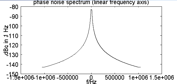
Fig 1: The phase noise spectrum used in the example
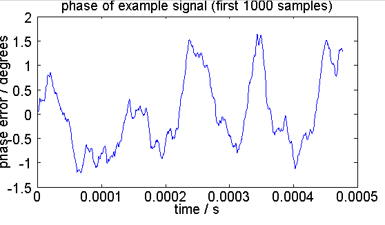
Fig. 2: Phase error observed on the generated example signal
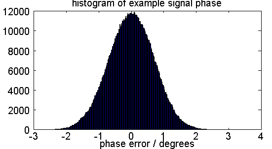
Fig. 3: Statistical distribution of phase error in the example signal
References:
[1] Basics of Phase noise and Jitter; Asad Abidi
[2] Wikipedia: Phase_noise
[3] Characterization of Frequency and Phase noise
How to run the code snippet:
Save as pn_snippet.m and call as pn_snippet
Tested on Matlab and OctaveForge
% ****************************************************************
% RMS phase error from phase noise spectrum
% Markus Nentwig, 2011
%
% - integrates RMS phase error from a phase noise power spectrum
% - generates an example signal and determines the RMS-average
%   phase error (alternative method)
% ****************************************************************
function pn_snippet()
    close all;

    % ****************************************************************
    % Phase noise spectrum model
    % --------------------------
    % Notes:
    % - Generally, a phase noise spectrum tends to follow
    %   |H(f)| = c0 + c1 f^n1 + c2 f^n2 + c3 f^n3 + ...
    %   Therefore, linear interpolation should be performed in dB
    %   on a LOGARITHMIC frequency axis.
    % - Single-/double sideband definition:
    %   The phase noise model is defined for -inf <= f <= inf
    %   in other words, it contributes the given noise density at
    %   both positive AND negative frequencies.
    %   Assuming a symmetrical PN spectrum, the model is evaluated
    %   for |f| => no need to explicitly write out the negative frequency
    %   side.
    % ****************************************************************

    % PN model
    % first column:
    %   frequency offset
    % second column:
    %   spectral phase noise density, dB relative to carrier in a 1 Hz
    %   observation bandwidth

    d = [0 -80
         10e3 -80
         1e6 -140
         9e9 -140];
    f_Hz = d(:, 1) .';
    g_dBc1Hz = d(:, 2) .' -3;

    % get RMS phase error by integrating the power spectrum
    % (alternative 1)
    e1_degRMS = integratePN_degRMS(f_Hz, g_dBc1Hz)

    % get RMS phase error based on a test signal
    % (alternative 2)
    n = 2 ^ 20;
    deltaF_Hz = 2;
    e2_degRMS = simulatePN_degRMS(f_Hz, g_dBc1Hz, n, deltaF_Hz)
end

% ****************************************************************
% Integrate the RMS phase error from the power spectrum
% ****************************************************************
function r = integratePN_degRMS(f1_Hz, g1_dBc1Hz)
    1;
    % integration step size
    deltaF_Hz = 100;

    % list of integration frequencies
    f_Hz = deltaF_Hz:deltaF_Hz:5e6;

    % interpolate spectrum on logarithmic frequency, dB scale
    % unit is dBc in 1 Hz, relative to a unity carrier
    fr_dB = interp1(log(f1_Hz+eps), g1_dBc1Hz, log(f_Hz+eps), 'linear');

    % convert to power in 1 Hz, relative to a unity carrier
    fr_pwr = 10 .^ (fr_dB/10);

    % scale to integration step size
    % unit: power in deltaF_Hz, relative to unity carrier
    fr_pwr = fr_pwr * deltaF_Hz;

    % evaluation frequencies are positive only
    % phase noise is two-sided
    % (note the IEEE definition: one-half the double sideband PSD)
    fr_pwr = fr_pwr * 2;

    % sum up relative power over all frequencies
    pow_relToCarrier = sum(fr_pwr);

    % convert the phase noise power to an RMS magnitude, relative to the carrier
    pnMagnitude = sqrt(pow_relToCarrier);

    % convert from radians to degrees
    r = pnMagnitude * 180 / pi;
end

% ****************************************************************
% Generate a PN signal with the given power spectrum and determine
% the RMS phase error
% ****************************************************************
function r = simulatePN_degRMS(f_Hz, g_dBc1Hz, n, deltaF_Hz);
    A = 1; % unity amplitude, arbitrary

    % indices of positive-frequency FFT bins.
    % Does not include DC
    ixPos = 2:(n/2);

    % indices of negative-frequency FFT bins.
    % Does not include the bin on the Nyquist limit
    assert(mod(n, 2) == 0, 'n must be even');
    ixNeg = n - ixPos + 2;

    % Generate signal in the frequency domain
    sig = zeros(1, n);
    % positive frequencies
    sig(ixPos) = randn(size(ixPos)) + 1i * randn(size(ixPos));
    % for purely real-valued signal: conj()
    % for purely imaginary-valued signal such as phase noise: -conj()
    % Note:
    %   Small-signals are assumed. For higher "modulation indices",
    %   phase noise would become a circle in the complex plane
    sig(ixNeg) = -conj(sig(ixPos));

    % normalize energy to unity amplitude A per bin
    sig = sig * A / RMS(sig);

    % normalize energy to 0 dBc in 1 Hz
    sig = sig * sqrt(deltaF_Hz);

    % frequency vector corresponding to the FFT bins (0, positive, negative)
    fb_Hz = FFT_freqbase(n, deltaF_Hz);

    % interpolate phase noise spectrum on frequency vector
    % interpolate dB on logarithmic frequency axis
    H_dB = interp1(log(f_Hz+eps), g_dBc1Hz, log(abs(fb_Hz)+eps), 'linear');

    % dB => magnitude
    H = 10 .^ (H_dB / 20);

    % plot on linear f axis
    figure(); hold on;
    plot(fftshift(fb_Hz), fftshift(mag2dB(H)), 'k');
    xlabel('f/Hz'); ylabel('dBc in 1 Hz');
    title('phase noise spectrum (linear frequency axis)');

    % plot on logarithmic f axis
    figure(); hold on;
    ix = find(fb_Hz > 0);
    semilogx(fb_Hz(ix), mag2dB(H(ix)), 'k');
    xlabel('f/Hz'); ylabel('dBc in 1 Hz');
    title('phase noise spectrum (logarithmic frequency axis)');

    % apply frequency response to signal
    sig = sig .* H;

    % add carrier
    sig (1) = A;

    % convert to time domain
    td = ifft(sig);

    % determine phase
    % for an ideal carrier, it would be zero
    % any deviation from zero is phase error
    ph_deg = angle(td) * 180 / pi;

    figure();
    ix = 1:1000;
    plot(ix / n / deltaF_Hz, ph_deg(ix));
    xlabel('time / s');
    ylabel('phase error / degrees');
    title('phase of example signal (first 1000 samples)');

    figure();
    hist(ph_deg, 300);
    title('histogram of example signal phase');
    xlabel('phase error / degrees');

    % RMS average
    % note: exp(1i*x) ~ x
    %       as with magnitude, power/energy is proportional to phase error squared
    r = RMS(ph_deg);

    % knowing that the signal does not have an amplitude component, we can alternatively
    % determine the RMS phase error from the power of the phase noise component

    % exclude carrier:
    sig(1) = 0;

    % 3rd alternative to calculate RMS phase error
    rAlt_deg = sqrt(sig * sig') * 180 / pi
end

% gets a vector of frequencies corresponding to n FFT bins, when the
% frequency spacing between two adjacent bins is deltaF_Hz
function fb_Hz = FFT_freqbase(n, deltaF_Hz)
    fb_Hz = 0:(n - 1);
    fb_Hz = fb_Hz + floor(n / 2);
    fb_Hz = mod(fb_Hz, n);
    fb_Hz = fb_Hz - floor(n / 2);
    fb_Hz = fb_Hz * deltaF_Hz;
end

% Root-mean-square average
function r = RMS(vec)
    r = sqrt(vec * vec' / numel(vec));
end

% convert a magnitude to dB
function r = mag2dB(vec)
    r = 20*log10(abs(vec) + eps);
end


