Narrow-band moving-average decimator, one addition/sample

Decimation for narrow-band signals by averaging

It is usually not practical to implement filters with a bandwidth many orders of magnitude below the sampling rate. For example, an application might demand the recovery of a "time-varying DC component" for frequencies < 3 Hz from a signal sampled at audio-frequency rates.

A straightforward filter design becomes inefficient and numerically instable. Instead, the signal should be decimated to a lower rate, where the filter can be implemented much more efficiently.

A lowpass response is needed to prevent aliasing from high frequency components of the input signal that do not "fit" into the lower rate of the decimated output signal.

Generally, this boils down to a multi-rate filter design task, and there is no single "best" solution. For example, one well-known approach is the CIC structure, but its implementation is not completely trivial.

One particular solution is to simply average n samples. Conceptually, this is equivalent to a rectangular moving average filter in combination with decimation.

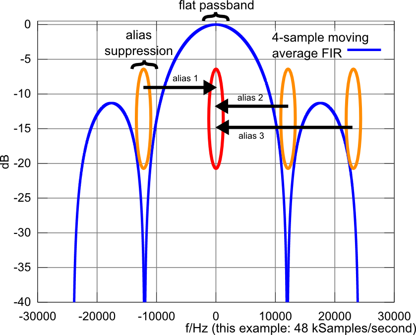
As the following picture shows (example: n=4), an averaging window with a length of n samples creates n notches in the frequency response that happen to fall exactly on those frequencies that would alias to 0 Hz after decimation by n. For signals that occupy only a narrow bandwidth in the output signal, relative to the output sampling rate, the filter gives good rejection of unwanted aliases.

Note that also other regions than those marked in orange circles will cause alias products. However, those products appear at frequencies in the output signal that do not overlap with the wanted signal bandwidth. They can be removed using a conventional filter on the low-rate signal.

Code snippet:

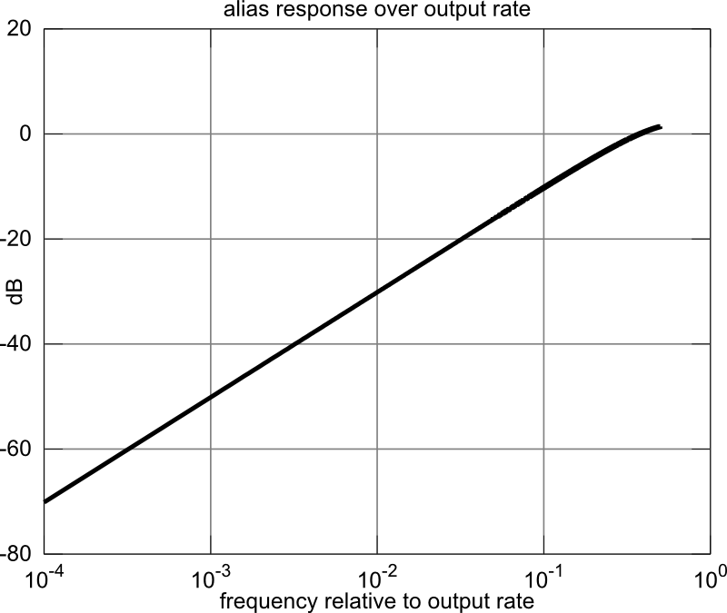
The Matlab program calculates the passband- and alias-response for a given n. The alias level is evaluated for an assumed equal power density at all out-of-band frequencies. In most application, this is a quite pessimistic assumption, and the following line

sAlias = s; sAlias(find(abs(fb) >= rateIn_Hz / decimationFactor / 2)) = 1;

could be edited to generate a more realistic out-of-band signal spectrum.

It plots charts for the passband flatness and alias response.

"Alias rejection"

The term "alias rejection" is not well defined. The reported number is meant as an order-of-magnitude estimate only.
Using the code snippet, aliases from all bands add coherently, as would be applicable to impulse-like noise.
For an additive white Gaussian noise-type unwanted signal component, the reported number can be expected to be somewhat pessimistic, as the unwanted signal components in different alias bands will be uncorrelated with each other.

The plot shows an example:

Implementation of the filter:

#define DECIM (100)

double acc = 0.0;
while (1){
   int ix;
   for(ix = DECIM; ix > 0; --ix){
      acc += getInputSample();
   } /* for */
   writeOutputSample(acc / (double)DECIM);
   acc = 0.0;
} /* while */

The implementation requires only a single addition per input sample, which is a benefit especially on general-purpose CPUs or microcontrollers, where multiplications are more expensive than additions.

Running the code snippet

Copy to eval_design.m and run eval_design from the command line.

Usage

• For a known wanted signal bandwidth and sampling rate, find the highest decimation factor n that results in tolerable aliasing and / or in-band distortion. If further decimation is required, it can be implemented with a conventional filter (which becomes increasingly efficient as its input rate decreases).

• Design a digital filter at the decimated rate that implements the desired frequency response and removes aliases between the wanted signal bandwidth and the sampling rate of the output signal.

Note: Since implementing a filter at the low, decimated rate is usually not very CPU-intensive, it may be a good idea to equalize the passband response at the same time.
The code snippet below calculates a frequency response that can be used directly as input to a FIR filter design algorithm such as this one.

% *************************************************
% Moving average decimator 
%
% A decimator for narrow-band signals (~5 % or less bandwidth occupation) 
% can be implemented as follows:
%
% #define DECIM (100)
% double acc = 0.0;
% while (1){
%    int ix;
%    for(ix = DECIM; ix > 0; --ix){
%       acc += getInputSample();
%    } /* for */
%    writeOutputSample(acc / (double)DECIM);
%    acc = 0.0;
% } /* while */
%
% It is conceptually identical to a moving average filter
% http://www.dspguide.com/ch15/4.htm combined with a decimator
%
% Note that the "moving" average jumps ahead in steps of the decimation
% factor. Intermediate output is decimated away, allowing for a very efficient 
% implementation.
% This program calculates the frequency response and alias response,
% based on the decimation factor and bandwidth of the processed signal.
% *************************************************    
function eval_design()
    decimationFactor = 100;
    rateIn_Hz = 48000;
    noDecim = false;
    
    % create illustration with sinc response
    %decimationFactor = 4; noDecim = true; 
    
    % *************************************************
    % signal source: Bandlimited test pulse
    % Does not contain energy in frequency ranges that 
    % cause aliasing
    % *************************************************
    s = zeros(1, 10000 * decimationFactor);    
    fb = FFT_frequencyBasis(numel(s), rateIn_Hz);
    
    % assign energy to frequency bins
    if noDecim
        sPass = ones(size(s));
    else
        sPass = s; sPass(find(abs(fb) < rateIn_Hz / decimationFactor / 2)) = 1;
    end
    sAlias = s; sAlias(find(abs(fb) >= rateIn_Hz / decimationFactor / 2)) = 1;
    
    % convert to time domain
    sPass = fftshift(real(ifft(sPass)));
    sAlias = fftshift(real(ifft(sAlias)));

    % *************************************************    
    % plot spectrum at input
    % *************************************************    
    pPass = {};
    pPass = addPlot(pPass, sPass, rateIn_Hz, 'k', 5, ...
                    'input (passband response)');
    pAlias = {};
    pAlias = addPlot(pAlias, sAlias, rateIn_Hz, 'k', 5, ...
                     'input (alias response)');    
        
    % *************************************************    
    % impulse response
    % *************************************************    
    h = zeros(size(s));
    h (1:decimationFactor) = 1; 
    if noDecim
        h = h / decimationFactor;
        decimationFactor = 1;
    end
    
    % cyclic convolution between signal and impulse response
    sPass = real(ifft(fft(sPass) .* fft(h)));
    sAlias = real(ifft(fft(sAlias) .* fft(h)));
    
    % decimation
    sPass = sPass(decimationFactor:decimationFactor:end);
    sAlias = sAlias(decimationFactor:decimationFactor:end);
    rateOut_Hz = rateIn_Hz / decimationFactor;
    
    % *************************************************    
    % plot spectrum
    % *************************************************    
    pPass = addPlot(pPass, sPass, rateOut_Hz, 'b', 3, ...
                    'decimated (passband response)');
    figure(1); clf; grid on; hold on;
    doplot(pPass, sprintf('passband frequency response over input rate, decim=%i', decimationFactor));
    
    pAlias = addPlot(pAlias, sAlias, rateOut_Hz, 'b', 3, ...
                     'decimated (alias response)');
    figure(2); clf; grid on; hold on;
    doplot(pAlias, sprintf('alias frequency response over input rate, decim=%i', decimationFactor));

    % *************************************************    
    % plot passband ripple
    % *************************************************    
    fb = FFT_frequencyBasis(numel(sPass), 1);
    fr = 20*log10(abs(fft(sPass) + eps));
    ix = find(fb > 0);

    figure(3); clf;
    h = semilogx(fb(ix), fr(ix), 'k');
    set(h, 'lineWidth', 3);
    ylim([-3, 0]);
    title(sprintf('passband gain over output rate, decim=%i', decimationFactor));
    xlabel('frequency relative to output rate');
    ylabel('dB'); grid on;
    
    % *************************************************    
    % plot alias response
    % *************************************************    
    fb = FFT_frequencyBasis(numel(sAlias), 1);
    fr = 20*log10(abs(fft(sAlias) + eps));
    ix = find(fb > 0);
    
    figure(4); clf;
    h = semilogx(fb(ix), fr(ix), 'k');
    set(h, 'lineWidth', 3);
    %    ylim([-80, -20]);
    title(sprintf('alias response over output rate, decim=%i', decimationFactor));
    xlabel('frequency relative to output rate');
    ylabel('dB'); grid on;    
end

% ************************************
% put frequency response plot data into p
% ************************************
function p = addPlot(p, s, rate, plotstyle, linewidth, legtext)
    p{end+1} = struct('sig', s, 'rate', rate, 'plotstyle', plotstyle, 'linewidth', linewidth, 'legtext', legtext);
end

% ************************************
% helper function, plot data in p
% ************************************
function doplot(p, t)
    leg = {};
    for ix = 1:numel(p)
        pp = p{ix};        
        fb = FFT_frequencyBasis(numel(pp.sig), pp.rate);
        fr = 20*log10(abs(fft(pp.sig) + eps));
        h = plot(fftshift(fb), fftshift(fr), pp.plotstyle);
        set(h, 'lineWidth', pp.linewidth);
        xlabel('f / Hz');
        ylabel('dB');
        leg{end+1} = pp.legtext;
    end
    legend(leg);
    title(t);
end

% ************************************
% calculates the frequency that corresponds to
% each FFT bin (negative, zero, positive)
% ************************************
function fb_Hz = FFT_frequencyBasis(n, rate_Hz)
    fb = 0:(n - 1);
    fb = fb + floor(n / 2);
    fb = mod(fb, n);
    fb = fb - floor(n / 2);
    fb = fb / n; % now [0..0.5[, [-0.5..0[
    fb_Hz = fb * rate_Hz;
end