Filter-Bank Summation (FBS) Interpretation of the STFT
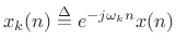
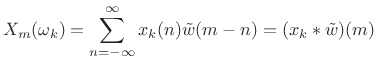
We can group the terms in the STFT definition differently to obtain
the filter-bank interpretation:
![$\displaystyle \sum_{n=-\infty}^\infty \underbrace{[ x(n)e^{-j\omega_k n}]}_{x_k(n)} w(n-m)$](http://www.dsprelated.com/josimages_new/sasp2/img1538.png)
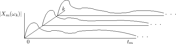
As will be explained further below (and illustrated further in Figures 9.3, 9.4, and 9.5), under the filter-bank interpretation, the spectrum of
Expanding on the previous paragraph, the STFT (9.2) is computed by the following operations:
- Frequency-shift
 by
by  to get
 .
.
- Convolve
 with
with
 to get
 :
:
(10.3)
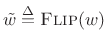
Note that the STFT analysis window ![]() is now interpreted as (the flip
of) a lowpass-filter impulse response. Since the analysis window
is now interpreted as (the flip
of) a lowpass-filter impulse response. Since the analysis window ![]() in the STFT is typically symmetric, we usually have
in the STFT is typically symmetric, we usually have
![]() .
This filter is effectively frequency-shifted to provide each channel
bandpass filter. If the cut-off frequency of the window transform is
.
This filter is effectively frequency-shifted to provide each channel
bandpass filter. If the cut-off frequency of the window transform is
![]() (typically half a main-lobe width), then each channel
signal can be downsampled significantly. This downsampling factor is
the FBS counterpart of the hop size
(typically half a main-lobe width), then each channel
signal can be downsampled significantly. This downsampling factor is
the FBS counterpart of the hop size ![]() in the OLA context.
in the OLA context.
Figure 9.3 illustrates the filter-bank interpretation for ![]() (the ``sliding STFT''). The input signal
(the ``sliding STFT''). The input signal ![]() is frequency-shifted
by a different amount for each channel and lowpass filtered by the
(flipped) window.
is frequency-shifted
by a different amount for each channel and lowpass filtered by the
(flipped) window.
![\begin{psfrags}
% latex2html id marker 23871\psfrag{w}{\Large$\protect\hbox{\sc Flip}(w)$}\psfrag{x(n)}{\LARGE$x(n)$}\psfrag{X0}{\LARGE$X_n(\omega_{\scriptscriptstyle 0}$)}\psfrag{X1}{\LARGE$X_n(\omega_{\scriptscriptstyle 1}$)}\psfrag{XNm1}{\LARGE$X_n(\omega_{\scriptscriptstyle {N}-1})$}\psfrag{ejw0}{\huge$e^{-j\omega_{\scriptscriptstyle 0}n}$}\psfrag{ejw1}{\huge$e^{-j\omega_{\scriptscriptstyle 1}n}$}\psfrag{ejwNm1}{\huge$e^{-j\omega_{\scriptscriptstyle {N-1}}n}$}\psfrag{dR}{\LARGE$\downarrow R$}\psfrag{X}{\LARGE$\times$}\begin{figure}[htbp]
\includegraphics[width=3in]{eps/fbs1}
\caption{Sliding STFT analysis filter bank.
The $k$th channel of the filter bank computes
$X_n(\omega_k)=(x_k\ast \hbox{\sc Flip}{w})(n)$, where $x_k(n)\isdeftext
x(n)\exp(-j\omega_k n)$.
}
\end{figure}
\end{psfrags}](http://www.dsprelated.com/josimages_new/sasp2/img1552.png)
Next Section:
FBS and Perfect Reconstruction
Previous Section:
Overlap-Add (OLA) Interpretation of the STFT