


Sinusoids
A sinusoid is any function having the following form:

An example is plotted in Fig.4.1.
The term ``peak amplitude'' is often shortened to ``amplitude,'' e.g.,
``the amplitude of the tone was measured to be 5 Pascals.'' Strictly
speaking, however, the amplitude of a signal ![]() is its instantaneous
value
is its instantaneous
value ![]() at any time
at any time ![]() . The peak amplitude
. The peak amplitude ![]() satisfies
satisfies
![]() . The ``instantaneous magnitude'' or simply
``magnitude'' of a signal
. The ``instantaneous magnitude'' or simply
``magnitude'' of a signal ![]() is given by
is given by ![]() , and the peak
magnitude is the same thing as the peak amplitude.
, and the peak
magnitude is the same thing as the peak amplitude.
The ``phase'' of a sinusoid normally means the ``initial phase'', but in some contexts it might mean ``instantaneous phase'', so be careful. Another term for initial phase is phase offset.
Note that Hz is an abbreviation for Hertz which physically means cycles per second. You might also encounter the notation cps (or ``c.p.s.'') for cycles per second (still in use by physicists and formerly used by engineers as well).
Since the sine function is periodic with period ![]() , the initial
phase
, the initial
phase
![]() is indistinguishable from
is indistinguishable from ![]() . As a result,
we may restrict the range of
. As a result,
we may restrict the range of ![]() to any length
to any length ![]() interval.
When needed, we will choose
interval.
When needed, we will choose
Note that the radian frequency ![]() is equal to the time
derivative of the instantaneous phase of the sinusoid:
is equal to the time
derivative of the instantaneous phase of the sinusoid:
![$\displaystyle \frac{d}{dt} [\omega t + \phi(t)] = \omega + \frac{d}{dt} \phi(t)
$](http://www.dsprelated.com/josimages_new/mdft/img380.png)
Example Sinusoids
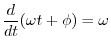
Figure 4.1 plots the sinusoid
![]() , for
, for ![]() ,
, ![]() ,
,
![]() , and
, and
![]() . Study the plot to make sure you understand the effect of
changing each parameter (amplitude, frequency, phase), and also note the
definitions of ``peak-to-peak amplitude'' and ``zero crossings.''
. Study the plot to make sure you understand the effect of
changing each parameter (amplitude, frequency, phase), and also note the
definitions of ``peak-to-peak amplitude'' and ``zero crossings.''
![\includegraphics[width=\twidth]{eps/sine}](http://www.dsprelated.com/josimages_new/mdft/img386.png)
A ``tuning fork'' vibrates approximately sinusoidally. An ``A-440'' tuning
fork oscillates at ![]() cycles per second. As a result, a tone recorded
from an ideal A-440 tuning fork is a sinusoid at
cycles per second. As a result, a tone recorded
from an ideal A-440 tuning fork is a sinusoid at ![]() Hz. The amplitude
Hz. The amplitude
![]() determines how loud it is and depends on how hard we strike the tuning
fork. The phase
determines how loud it is and depends on how hard we strike the tuning
fork. The phase ![]() is set by exactly when we strike the tuning
fork (and on our choice of when time 0 is). If we record an A-440 tuning
fork on an analog tape recorder, the electrical signal recorded on tape is
of the form
is set by exactly when we strike the tuning
fork (and on our choice of when time 0 is). If we record an A-440 tuning
fork on an analog tape recorder, the electrical signal recorded on tape is
of the form
As another example, the sinusoid at amplitude ![]() and phase
and phase ![]() (90 degrees)
is simply
(90 degrees)
is simply
Why Sinusoids are Important
Sinusoids arise naturally in a variety of ways:
One reason for the importance of sinusoids is that they are fundamental in physics. Many physical systems that resonate or oscillate produce quasi-sinusoidal motion. See simple harmonic motion in any freshman physics text for an introduction to this topic. The canonical example is the mass-spring oscillator.4.1
Another reason sinusoids are important is that they are eigenfunctions of linear systems (which we'll say more about in §4.1.4). This means that they are important in the analysis of filters such as reverberators, equalizers, certain (but not all) ``audio effects'', etc.
Perhaps most importantly, from the point of view of computer music research, is that the human ear is a kind of spectrum analyzer. That is, the cochlea of the inner ear physically splits sound into its (quasi) sinusoidal components. This is accomplished by the basilar membrane in the inner ear: a sound wave injected at the oval window (which is connected via the bones of the middle ear to the ear drum), travels along the basilar membrane inside the coiled cochlea. The membrane starts out thick and stiff, and gradually becomes thinner and more compliant toward its apex (the helicotrema). A stiff membrane has a high resonance frequency while a thin, compliant membrane has a low resonance frequency (assuming comparable mass per unit length, or at least less of a difference in mass than in compliance). Thus, as the sound wave travels, each frequency in the sound resonates at a particular place along the basilar membrane. The highest audible frequencies resonate right at the entrance, while the lowest frequencies travel the farthest and resonate near the helicotrema. The membrane resonance effectively ``shorts out'' the signal energy at the resonant frequency, and it travels no further. Along the basilar membrane there are hair cells which ``feel'' the resonant vibration and transmit an increased firing rate along the auditory nerve to the brain. Thus, the ear is very literally a Fourier analyzer for sound, albeit nonlinear and using ``analysis'' parameters that are difficult to match exactly. Nevertheless, by looking at spectra (which display the amount of each sinusoidal frequency present in a sound), we are looking at a representation much more like what the brain receives when we hear.
In-Phase & Quadrature Sinusoidal Components
From the trig identity
![]() , we have
, we have

From this we may conclude that every sinusoid can be expressed as the sum
of a sine function (phase zero) and a cosine function (phase ![]() ). If
the sine part is called the ``in-phase'' component, the cosine part can be
called the ``phase-quadrature'' component. In general, ``phase
quadrature'' means ``90 degrees out of phase,'' i.e., a relative phase
shift of
). If
the sine part is called the ``in-phase'' component, the cosine part can be
called the ``phase-quadrature'' component. In general, ``phase
quadrature'' means ``90 degrees out of phase,'' i.e., a relative phase
shift of ![]() .
.
It is also the case that every sum of an in-phase and quadrature component can be expressed as a single sinusoid at some amplitude and phase. The proof is obtained by working the previous derivation backwards.
Figure 4.2 illustrates in-phase and quadrature components
overlaid. Note that they only differ by a relative ![]() degree phase
shift.
degree phase
shift.
Sinusoids at the Same Frequency
An important property of sinusoids at a particular frequency is that they
are closed with respect to addition. In other words, if you take a
sinusoid, make many copies of it, scale them all by different gains,
delay them all by different time intervals, and add them up, you always get a
sinusoid at the same original frequency. This is a nontrivial property.
It obviously holds for any constant signal ![]() (which we may regard as
a sinusoid at frequency
(which we may regard as
a sinusoid at frequency ![]() ), but it is not obvious for
), but it is not obvious for ![]() (see
Fig.4.2 and think about the sum of the two waveforms shown
being precisely a sinusoid).
(see
Fig.4.2 and think about the sum of the two waveforms shown
being precisely a sinusoid).
Since every linear, time-invariant (LTI4.2) system (filter) operates by copying, scaling, delaying, and summing its input signal(s) to create its output signal(s), it follows that when a sinusoid at a particular frequency is input to an LTI system, a sinusoid at that same frequency always appears at the output. Only the amplitude and phase can be changed by the system. We say that sinusoids are eigenfunctions of LTI systems. Conversely, if the system is nonlinear or time-varying, new frequencies are created at the system output.
To prove this important invariance property of sinusoids, we may
simply express all scaled and delayed sinusoids in the ``mix'' in
terms of their in-phase and quadrature components and then add them
up. Here are the details in the case of adding two sinusoids having
the same frequency. Let ![]() be a general sinusoid at frequency
be a general sinusoid at frequency
![]() :
:
![\begin{eqnarray*}
y(t) &\isdef & g_1 x(t-t_1) + g_2 x(t-t_2) \\
&=& g_1 A \sin[\omega (t-t_1) + \phi]
+ g_2 A \sin[\omega (t-t_2) + \phi]
\end{eqnarray*}](http://www.dsprelated.com/josimages_new/mdft/img411.png)
Focusing on the first term, we have
![\begin{eqnarray*}
g_1 A \sin[\omega (t-t_1) + \phi]
&=&
g_1 A \sin[\omega t + (...
...omega t) \\
&\isdef & A_1 \cos(\omega t) + B_1 \sin(\omega t).
\end{eqnarray*}](http://www.dsprelated.com/josimages_new/mdft/img412.png)
We similarly compute
Constructive and Destructive Interference
Sinusoidal signals are analogous to monochromatic laser light. You
might have seen ``speckle'' associated with laser light, caused by
destructive interference of multiple reflections of the light beam. In
a room, the same thing happens with sinusoidal sound. For example,
play a simple sinusoidal tone (e.g., ``A-440''--a sinusoid at
frequency ![]() Hz) and walk around the room with one ear
plugged. If the room is reverberant you should be able to find places
where the sound goes completely away due to destructive interference.
In between such places (which we call ``nodes'' in the soundfield),
there are ``antinodes'' at which the sound is louder by 6
dB (amplitude doubled--decibels (dB) are reviewed in Appendix F)
due to constructive interference. In a diffuse reverberant
soundfield,4.3the distance between nodes is on the order of a wavelength
(the ``correlation distance'' within the random soundfield).
Hz) and walk around the room with one ear
plugged. If the room is reverberant you should be able to find places
where the sound goes completely away due to destructive interference.
In between such places (which we call ``nodes'' in the soundfield),
there are ``antinodes'' at which the sound is louder by 6
dB (amplitude doubled--decibels (dB) are reviewed in Appendix F)
due to constructive interference. In a diffuse reverberant
soundfield,4.3the distance between nodes is on the order of a wavelength
(the ``correlation distance'' within the random soundfield).
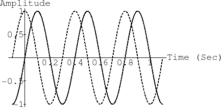
The way reverberation produces nodes and antinodes for sinusoids in a room is illustrated by the simple comb filter, depicted in Fig.4.3.4.4
Since the comb filter is linear and time-invariant, its response to a
sinusoid must be sinusoidal (see previous section).
The feedforward path has gain ![]() , and the delayed signal is scaled by
, and the delayed signal is scaled by ![]() .
With the delay set to one period, the sinusoid coming out of the delay
line constructively interferes with the sinusoid from the
feed-forward path, and the output amplitude is therefore
.
With the delay set to one period, the sinusoid coming out of the delay
line constructively interferes with the sinusoid from the
feed-forward path, and the output amplitude is therefore
![]() .
In the opposite extreme case, with the delay set to
half a period, the unit-amplitude sinusoid coming out of the
delay line destructively interferes with the sinusoid from the
feed-forward path, and the output amplitude therefore drops to
.
In the opposite extreme case, with the delay set to
half a period, the unit-amplitude sinusoid coming out of the
delay line destructively interferes with the sinusoid from the
feed-forward path, and the output amplitude therefore drops to
![]() .
.
Consider a fixed delay of ![]() seconds for the delay line in
Fig.4.3. Constructive interference happens at all
frequencies for which an exact integer number of periods fits
in the delay line, i.e.,
seconds for the delay line in
Fig.4.3. Constructive interference happens at all
frequencies for which an exact integer number of periods fits
in the delay line, i.e.,
![]() , or
, or ![]() , for
, for
![]() . On the other hand, destructive interference
happens at all frequencies for which there is an odd number of
half-periods, i.e., the number of periods in the
delay line is an integer plus a half:
. On the other hand, destructive interference
happens at all frequencies for which there is an odd number of
half-periods, i.e., the number of periods in the
delay line is an integer plus a half:
![]() etc., or,
etc., or,
![]() , for
, for
![]() . It is quick
to verify that frequencies of constructive interference alternate with
frequencies of destructive interference, and therefore the
amplitude response of the comb filter (a plot of gain versus
frequency) looks as shown in Fig.4.4.
. It is quick
to verify that frequencies of constructive interference alternate with
frequencies of destructive interference, and therefore the
amplitude response of the comb filter (a plot of gain versus
frequency) looks as shown in Fig.4.4.
![\includegraphics[width=4in,height=2.0in]{eps/combfilterFR}](http://www.dsprelated.com/josimages_new/mdft/img424.png)
The amplitude response of a comb filter has a ``comb'' like shape,
hence the name.4.5 It looks even more like a comb on a dB
amplitude scale, as shown in Fig.4.5. A dB scale is
more appropriate for audio applications, as discussed in
Appendix F. Since the minimum gain is
![]() , the nulls
in the response reach down to
, the nulls
in the response reach down to ![]() dB; since the maximum gain is
dB; since the maximum gain is
![]() , the maximum in dB is about 6 dB. If the feedforward gain
were increased from
, the maximum in dB is about 6 dB. If the feedforward gain
were increased from ![]() to
to ![]() , the nulls would extend, in
principle, to minus infinity, corresponding to a gain of zero
(complete cancellation). Negating the feedforward path would shift
the curve left (or right) by 1/2 Hz, placing a minimum at
dc4.6 instead of a peak.
, the nulls would extend, in
principle, to minus infinity, corresponding to a gain of zero
(complete cancellation). Negating the feedforward path would shift
the curve left (or right) by 1/2 Hz, placing a minimum at
dc4.6 instead of a peak.
![\includegraphics[width=4in,height=2.0in]{eps/combfilterFRDB}](http://www.dsprelated.com/josimages_new/mdft/img428.png)
Sinusoid Magnitude Spectra
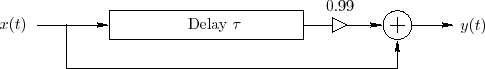
A sinusoid's frequency content may be graphed in the frequency domain as shown in Fig.4.6.
An example of a particular sinusoid graphed in Fig.4.6 is given by
Figure 4.6 can be viewed as a graph of the magnitude
spectrum of ![]() , or its spectral magnitude representation
[44]. Note that the spectrum consists of two components
with amplitude
, or its spectral magnitude representation
[44]. Note that the spectrum consists of two components
with amplitude ![]() , one at frequency
, one at frequency ![]() Hz and the other at
frequency
Hz and the other at
frequency ![]() Hz.
Hz.
Phase is not shown in Fig.4.6 at all. The phase of the components could be written simply as labels next to the magnitude arrows, or the magnitude arrows can be rotated ``into or out of the page'' by the appropriate phase angle, as illustrated in Fig.4.16.
Next Section:
Exponentials
Previous Section:
Euler_Identity Problems


