


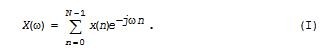
FFT Interpolation Based on FFT Samples: A Detective Story With a Surprise Ending
This blog presents several interesting things I recently learned regarding the estimation of a spectral value located at a frequency lying between previously computed FFT spectral samples. My curiosity about this FFT interpolation process was triggered by reading a spectrum analysis paper written by three astronomers [1].
My fixation on one equation in that paper led to the creation of this blog.
Background
The notion of FFT interpolation is straightforward to describe. That is, for example, given an N = 16 sample x(n) time-domain sequence shown in Figure 1(a), performing an N = 16 point FFT on x(n) produces the |X(m)| magnitude of samples shown by the red dots in Figure 1(b). The blue dashed curve in Figure 1(b) is the magnitude of the discrete-time Fourier transform (DTFT) of x(n), what I like to call the "true spectrum" of x(n).
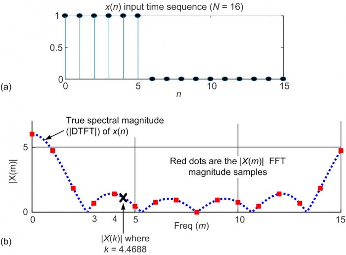
Figure 1: (a) An x(n) time sequence; (b) the spectral magnitude of x(n).
The process of FFT interpolation is estimating an X(k) spectral value at, for example, a non‑integer frequency of k = 4.4688 lying between the m = 4 and m = 5 FFT samples. The magnitude of X(k) is marked by the bold 'x' in Figure 1(b).
An X(k)Estimation Equation That Does Not Work
Reference [1] presents the following equation for computing a single X(k) spectral value based on N FFT samples:
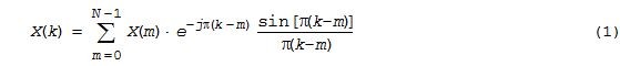
where:
- N = the number of x(n) input samples and the number of FFT samples
- X(m) = the original FFT samples, the FFT of x(n)
- m = the frequncy-domain integer index of X(m) where 0 ≤ m ≤ N-1
- k = the non-integer "FFT bin-like" frequency value of the desired spectral value
- j = sqrt(-1)
To avoid overwhelming the reader with too many algebra equations, I've included the derivation of Eq. (1) in Appendix A of the downloadable PDF file associated with this blog.
Not having seen Eq. (1) before I decided to model it using MATLAB software. Plugging my Figure 1(b) complex-valued X(m) FFT samples and k = 4.4688 into Eq. (1) I computed an XRef.[1](4.4688) value of:
XRef.[1](4.4688) = -1.1023 -j1.1053.
Next, padding the x(n) time sequence with lots of zero-valued samples I computed a finer-granularity spectrum shown by the blue dashed curve in Figure 1(b). From that finer-resolution spectrum I learned the true value of XTrue(4.4688) is:
XTrue(4.4688) = 0.3537 -j1.0489
which is not even close to the above XRef.[1](4.4688) spectral value computed using Eq. (1)! So what's going on here(!)?Knowing that my home-grown MATLAB code is about as reliable as the paper towel dispenser in the Men's Room, I asked our DSP colleague Neil Robertson to implement Eq. (1) using my above x(n) sequence and a value of k = 4.4688. Neil graciously agreed and his MATLAB code produced the same incorrect XRef.[1](4.4688) = ‑1.1023 ‑j1.1053 that I obtained.
So now it seems likely that Eq. (1) is not valid. But if that is true, how could the three authors of Reference [1] have missed that error? That was the mystery I set out to solve.
We'll revisit Eq. (1) later in this blog and learn something interesting in our quest to understand that equation.An X(k) Estimation Equation That Does Work
Knowing that Eq. (1) is questionable I started looking through my DSP books to find a valid FFT interpolation formula. In an old out-of-print book written by two DSP pioneers [2], I found the following expression for computing the spectral value at non-integer frequency k based on N X(m) FFT samples:
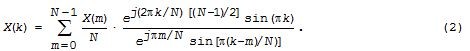
Equation (2) produces correct FFT interpolation results and its derivation is given in Appendix B of the downloadable PDF file. Using [2]'s z-transform derivation approach I performed a modified derivation to obtain the following computationally simpler FFT interpolation equation that also works just fine:
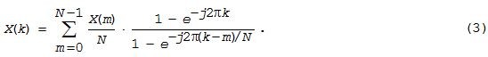
My derivation of Eq. (3) is presented in Appendix C of the downloadable PDF file.
Quiz of the Day
Equation (3) is a correct way to compute an interpolated X(k) value, but look at it carefully. Before continuing, do you see a way to reduce the number of arithmetic operations needed to compute a single X(k) value? Did you notice that neither the numerator nor the 1/N factor inside the summation in Eq. (3) are functions of m? That fact allows us to move them both outside the summation giving us:

Equation (4) has a significantly reduced computational workload relative to that of Eq. (3) as we shall see. Don't feel bad if you didn't foresee those beneficial simplifications leading to Eq. (4). Neither did I—while writing this blog I found those slick algebraic moves in [3].
So now, Eq. (4) is my preferred method for computing a single interpolated X(k) spectral value based on N FFT samples. Now that we have a workable Eq. (4), let's briefly revisit the suspicious Eq. (1).Here's What's Wrong With Eq. (1)
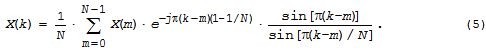
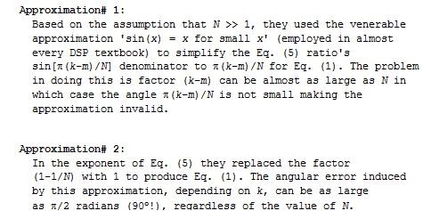
If you download the PDF file associated with this blog, in its Appendix A you'll see the published derivation of the troublesome Eq. (1). One intermediate step in that derivation, my Eq. (A‑5) repeated here as Eq. (5), produces the following expression for our desired X(k) as:
Examples of the errors of those two approximations are shown in Figure 2.
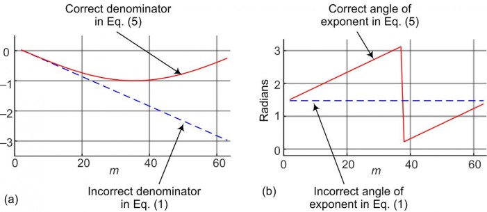
Figure 2: Approximations' errors, versus m, when k = 2.4688 and N = 64: (a) Approximation# 1 error; (b) Approximation# 2 error.
Analyzing the errors induced by those two approximations solves the mystery of why Eq. (1) is flawed. By the way, I've modeled Eq. (1) for values of N = 16 out to N = 16384 with no improvement in its accuracy for larger N. Next we discuss the computational costs of this blog's FFT interpolation equations.
Computational Workload Comparisons
It's enlightening to compare the necessary arithmetic operations needed to implement the correct FFT interpolation equations given in this blog.
Assuming we have previously computed and stored all the constant factors in our equations that are not functions of k or m, Table 1 shows the reduction in the necessary computations needed by Eqs. (4) and (5) relative to Eqs. (2) and (3). (In Table 1, a "Trigonometric Computation" means computing the sine or cosine of some given angle.)
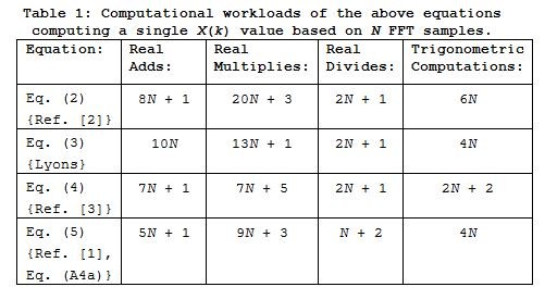
We remind the reader that Trigonometric Computations and Real Divides are far more computationally costly than Real Adds and Real Multiplies.
Here's the "Surprise Ending" To This Blog
While struggling to create Table 1 it finally hit me! The fastest way to compute a single interpolated FFT spectral sample at frequency k is to merely compute a brute force N‑point DFT of the original x(n) time samples using:
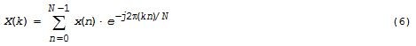
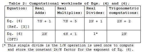
From Table 2 we see that Eq. (6) requires significantly fewer arithmetic operations—notably eliminating 2N of those costly 'Real Divides'—than Eq. (4).
Conclusions
I presented an X(k) FFT interpolation equation published in the literature, Eq. (1), for computing a single X(k) spectral value based on N FFT samples, where frequency k is not an integer. Equation (1) is not valid and I showed why that is so. (I remain troubled by this and perhaps someone can prove me wrong.) Next I presented four different expressions, Eq. (2) through Eq. (5), for computing an X(m) sample and compared their computational costs. Finally I realized the most efficient method for computing a single X(k) sample is to simply perform an N‑point DFT using Eq. (6).
I apologize for this blog being so lengthy. I didn't have the time to make it shorter.
Postscript [April 26, 2018]: My original typographical error pointed out in DerekR's April 24th 2018 post has been corrected in the above blog and corrected in the updated "Version 3" PDF file associated with this blog.
References
[1] S. Ransom, S. Eikenberry, and J. Middleditch, "Fourier Techniques For Very Long Astrophysical Time-Series Analysis", The Astronomical Journal, Sept. 2002, Section 4.1, pp. 1796. [http://iopscience.iop.org/article/10.1086/342285/pdf]
[2] L. Rabiner and B. Gold, Theory and Application of Digital Signal Processing, Prentice Hall, Upper Saddle River, New Jersey, 1975, p. 54.
[3] J. Proakis and D. Manolakis, Digital Signal Processing-Principles, Algorithms, and Applications, 3rd Ed., Prentice Hall, Upper Saddle River, New Jersey, 1996, pp. 408.


- Comments
- Write a Comment Select to add a comment
Hi Rick,
So I'm the primary author of the paper that you are discussing and I can guarantee you that Fourier Interpolation works extremely well! It has been used to help discover many hundreds of new pulsars.
One of the big issues here, I think, is that your Eqn 1 (my Eqn 29) was only derived to apply when N is very large (N larger than hundreds or thousands). But Eqn 29 isn't the interesting one. Eqn 30 in my paper is:
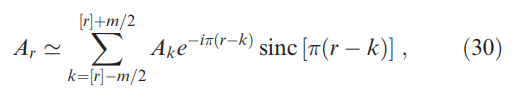
If N is large (again, that is a requirement), then you can interpolate your FFT at a non-integer frequency "r" to whatever precision you like, by summing ~m local Fourier amplitudes (integer freqs "k" surrounding freq "r"). For single-precision work, I usually use m of between 30-40.
The result of using this type of Fourier interpolation is exactly equivalent to zero-padding the original time series (if you do them equivalently). But if you only need small portions of the spectrum interpolated, Fourier interpolation via the above equation is hugely faster as it only needs a small number of operations.
Note that Eqn 30 is effectively a complex FIR filter, which means that we can also do the interpolation via correlations using the convolution theorem in the Fourier domain (using FFTs of small portions of the large-N FFT). And, in fact, that is exactly how my pulsar search software uses Eqn 30 during large-scale Fourier searches.
Let me know if you have any questions,
Scott Ransom
http://www.cv.nrao.edu/~sransom
I should also mention that the formula that I gave above only works if we are using the same definition of forward and reverse FFTs! For the version above, I assume that a forward FFT using a negative in the exponential. If you use the opposite sign convention, then some signs in Eqn 30 need flipped as well!

Hi Scott.
It's nice to hear from you. First I want to say congratulations on on your comprehensive paper. You guys are doing some fascinating signal processing. As time permits I hope to study your paper further to understand your novel curves in your Figure 1. (I've never seen anything like those curves before.)
I want to mention that a few years ago I was driving past the National Radio Astronomy Observatory (NRAO) facility near Los Alamos, NM. I could hardly believe my eyes when I saw that super large dish antenna there. I stopped my car by the front gate of that facility, got out and walked back-n-forth, but was afraid to walk into the facility unannounced. I so badly wanted to go in there and ask the engineers about 100 questions regarding the dish antenna and the signals it receives. (There was no guard at the front gate to stop me from entering, but all the "Warning" signs at the front gate scared me away.)
Scott, in your paper's Section 3.2.1 you discuss the important concept of "DFT scalloping loss." With that topic in mind, you might find the blog at:
https://www.dsprelated.com/showarticle/538.php
to be mildly interesting.
Hi Rick,
Yes, I have to admit that after I figured out that the DFT (or FFT) is simply a vector addition in the complex plane, I got very interested in that. It helped me understand much more about Fourier analysis.
And yes, that scalloping loss blog post is interesting. The scalloping issue is very important for pulsar astronomers as new pulsars almost never have spin periods (or their harmonics) that sit in integer frequency bins!
I'm hoping to find some time to investigate what you suggest are the two bad assumptions that resulted in Eqn 1. I'm pretty sure that 1) if N is large and 2) if the frequencies that you are interested in are not near the ends of the FFT (i.e. near zero or near the Nyquist freq) that things actually work out so that those approximations are OK (especially since you sum over a bunch of terms).
Note that that 2nd bit above, about not being near the ends of the FFT, is an important one.
Cheers,
Scott
Hi Scott.
Yes yes. Your concern regarding the behavior of Eq. (1) when the desired spectral estimate's frequency is near zero or Fs/2 Hz is valid.
Let's say we applied a real-valued pure sinusoidal input sequence, padded with lots of zero-valued samples, whose frequency is very near Fs/4 Hz to the DFT. The spectral magnitude results show a positive-freq |sin(x)/x|-like envelope and a negative-freq |sin(x)/x|-like envelope. Those |sin(x)/x| envelopes are very symmetrical in that their lower and upper sidelobes are roughly mirror images of each other.
Next we apply a real-valued pure sinusoidal input sequence, padded with lots of zero-valued samples, whose frequency is very near zero (or Fs/2) Hz to the DFT. The spectral magnitude results show a positive-freq distorted |sin(x)/x|-like envelope and a negative-freq distorted |sin(x)/x|-like envelope. Those |sin(x)/x| envelopes are "distorted" in that they are not symmetrical. Their lower and upper sidelobes are no longer mirror images of each other. I interpret that behavior to be caused by spectral leakage from the negative-freq spectral energy crossing the zero-Hz (or Fs/2-Hz) boundary and contaminating the positive-freq spectral components. Likewise I believe spectral
leakage from the positive-freq spectral energy crosses the zero-Hz
(or Fs/2) boundary and contaminates the negative-freq spectral components.
You already know this Scott, but what I'm sayin' is: The true shape of the positive-frequency spectral magnitude envelope of a real-valued sinusoidal sequence depends on the frequency of that sinusoid. When the sinusoid's frequency is near zero or Fs/2 Hz, the positive-freq magnitude envelope will NOT be a |sin(x)/x| curve. However, the larger the size of the DFT the more similar the spectral magnitude envelopes will be to a |sin(x)/x| curve.
I don't know if what I've written here makes sense, but in any case I'm agreeing with you Scott. Spectral estimation in the vicinity of zero Hz and Fs/2 Hz deserves contemplation and examination.
Yup. I completely agree.
For pulsar work, the FFTs we usually use are typically many millions of points long (sometimes even billions), and the frequencies of interest are nowhere near the edges. In that regime, the complex sinc-like response in the Fourier interpolation formula is *very* accurate. When dealing with short FFTs and or frequencies near the boundaries, that is definitely not the case as you have shown!

Interesting post Rick. Keep the good work up.
Your conclusion makes sense, Scott.
If we consider windowing in frequency domain, for example using blackman window,
this formula should work:
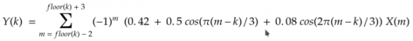
where Y(k) is windowed frequency domain value at fractional k, the phase is shifted to be centered at N/2 instead 0.
The true value at 4.4688 or any other non-integer frequency is zero. Anything else requires further explanation about the context of the time domain sequence.
Maybe it’s not as explicit as you would like but I thought it was obvious that the signal is zero for all other values of n.
And if we’re nitpicking, non-integer values being zero would only be true if the signal were periodic, which would also require further explanation about the context of the time domain sequence.
Hi dszabo. My blog's finite-length x(n) sequence only has 16 samples, x(0) -to- x(15). We can make NO assumptions regarding sample x(16) because sample x(16) does not exist. (I can make no assumptions regarding the ear drum inside Vladimir Putin's third ear because Vlad doesn't have a third ear.)
Perhaps I misunderstood the intention. I had assumed when you referenced the DTFT as the true spectrum and used zero-padding to increase spectral resolution that the signal is interpreted as having an infinite data set that is zero outside the dined range from 0 to 15
Hi dszabo.
Perhaps I misunderstood your post. If you are saying that my blog's 16-sample x(n) and another sequence whose first 16 samples are my x(n) samples followed by 100 zero-valued samples have the same DTFT, then I 100% agree with you.
I think what I’m trying to reconcile is that the DTFT is defined for an infinite data set, while the DFT is defined for a finite data set. In that sense, The only way I can get my head around the DTFT of a 16 or 116 point set of data is to say that the set is actually infinite and make an assumption about what the rest of it is. If you specify that all undefined points are zero, then it’s trivial to show that individual points in the spectrum are calculated as you described in this article.
Perhaps it’s a semantic or perceptual point, but I find it makes the most sense for me personally
Hello Stenz.
Well, ...in a 'discrete sequence only' context where only 16 X(m) FFT samples exist, X(4.4688) is not zero. In that context X(4.4688) does not exist! In that 'discrete sequence only' context my asking you what is the value of X(4.4688) is like asking you, "What day of the week follows Tuesday but is before Wednesday?"
Now in the broader contest of our world of algebra, we can think of a continuous function X(w) called the "discrete-time Fourier transform (DTFT) of an N-length x(n) sequence" defined by:
X(w) is x(n)'s z-transform evaluated on the z-plane's unit circle. In this context frequency w (omega) is continuous. We can write Eq. (I) on paper and think about X(w) but, because w is continuous, we cannot represent X(w) with any sort of data stored in the memory of a digital computer. The X(w) only exits as a scribble on paper and as an abstract idea in our brains.
However, using a computer we can evaluate Eq. (I)'s X(w) for a single specific value of w.
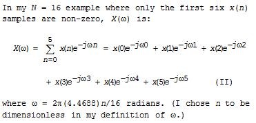
So I claim, for my blog's x(n), X(w) does exist and
X(2*pi*4.4688*n/16) = 0.3536 -j1.0489.
Stenz, you might next say to me, "Rick, without using all your algebraic mumbo-jumbo, prove to me that X(w) and X(2*pi*4.4688*n/16) exist." Such a challenge from you would invite contemplation on my part.
A DFT is an orthogonal transform which implies that x(n) is a periodic sequence.
Your DFT with non-integer frequency component is no longer orthogonal, and the interpolation only makes sense if x(n) is not periodic but zero anywhere outside the interval 0..N-1. Maybe I'm nitpicking, but I experience so much misunderstanding about DFT/FFT that I find it important to clarify.
How does the DFT being an orthogonal transform imply that x(n) is periodic? Wouldn’t it just imply the x(n) has a finite length?
Stenz, if you want to debate then let's debate, but let's make sure our words are crystal clear. Your first sentence (containing the word "implies") is vague. Please define the meaning of your phrase "periodic sequence." After doing that please tell me if your first sentence is claiming that the DFT can only be performed on what you have defined to be a "periodic sequence."
The first part of your second sentence puzzles me. What do you mean by a "DFT with a non-integer frequency component"? Have you ever encountered a sequence of DFT samples where that freq-domain sequence's index has non-integer values? I haven't.
I agree with you that there is "much misunderstanding about DFT/FFT" out there in the literature. My favorite example of a truly profound misunderstanding, from people who are swimming too far from the shores of sanity, is: "The DFT assumes its input sequence is periodic."
Well, you can DFT any data you want, periodic or not, but if you interpret the output as frequency content, there are only two cases that make sense: the underlying data is periodic, or it is zero padded on both ends towards infinity. In both cases the true spectrum is revealed, but only in the latter case the spectrum is a continuous function.
If you look at the x(n) and it's DFT in isolation, there is little sense in interpolating any non-integer frequency, there is as much justification saying it is zero as any other value - you just produce meaningless data out of thin air.
I asked you three questions hoping your answers would help me understand your April 17th post. Sadly, you didn't answer any of my questions.
I would say that either way something must be assumed about the time-domain sequence.
If you say that the value at the non-integer frequency is "zero", (or perhaps more correctly, not defined, as Rick says), then you are assuming the original time-domain sequence is periodic, as dszabo says.
But this is not stated in the blog.
I would have thought the most logical assumption is that the sequence is zero outside the shown range, in which case the DTFT shows the underlying frequency spectrum, and the DFT allows one to compute samples of this spectrum.
Hi Michael. These kinds of discussions regarding the DFT are interesting, often educational, and fun. (Did you have a look at my reply to dszabo's post?)
My blog's finite-length x(n) sequence
only has 16 samples, x(0) -to- x(15). We can compute a 16-point DFT of those samples without having to make any assumptions
regarding x(n). If you want to think about a time-domain sequence whose first 16 samples are my x(n) samples followed by 100 zero-valued samples, that's fine with me. But your new 116-sample time sequence, let's call it y(n), is not equal to my blog's 16-sample x(n) time sequence.
Everything I wrote in my blog strictly applies to, and only to, the 16-sample x(n) in Figure 1(a) of my blog.
Hi Rick,
I agree, for what seems like a simple transform on the surface, the DFT hides huge subtly and intrigue!
Apologies if my post appears to contradict anything in your blog, it was meant as a reply to Stenz's first post.
You say that you can compute a 16-point DFT without any assumptions about x(n) outside the range given, and I see where you're coming from on this now - the 16-point DFT takes in 16 samples, and that's it. Right?
I have a question: in what sense is the DTFT interpolating the DFT samples? If we only have 16 samples, what constraints are we applying that suggest the DTFT is the "correct" interpolation, rather than say a polynomial interpolation, or just a plain old fashioned linear interpolation between the points? Or even just saying that no interpolation is possible, since there is no value in-between the two points i.e. it could be like asking what integer is half-way between 2 and 3, according to a linear interpolation. Answer: none exists.
Hi Michael. I'm not ignoring you. I'm thinking about your "good question."
No problem, Rick - there's no rush. Usually I find my best thinking happens when I relax and reflect on such things.
Explanation for the failure of Eq. (1):
Eq. (1) is basically the frequency domain equivalent of the time domain Cardinal/Whittaker interpolation/reconstruction for a sampled time domain signal:
infiity
f(t) = sum [f(nT) * sin( pi*((t-nT)/T)/(pi*(t-nT)/T)] (a)
n = -infinity
as a sum of weighted sinc functions. Eq. (a) is a convolution of the sampled waveform f(nT) (a set of weighted impulses) with the impulse response of the ideal (rectangular) continuous time reconstruction filter.
However, note the limits of the summation - they go from -infinity to infinity, and note that the impulse response is (i) acausal, and (ii) infinite,
Now, we know that the basic assumption in the DFT is that the signals f(n) and F(m) in both domains are periodic with period N (the length of the transform), that is THEY ARE NOT FINITE in extent and any attempt to process them MUST recognize that fact. Then applying Eq. (a) to a time domain signal that is derived from an IDFT must include all of the periodic extensions of the output. A careful look at Eq. (a) will show that the contribution to the sum by the extensions decays slowly, and therefore we have to take many periodic extensions into account to come up with a reasonable approximation.
I won't do it here, but using the properties of the DFT (or the FT) can lead to Eq. (1) as a spectral interpolator similar in form to my Eq. (a), and the same condition applies: any attempt to evaluate an interpolated spectral value must include all (or at least a large number) of periodic extensions of F(m) in the sum. A single period will just not hack it :-)
To demonstrate this I wrote my own MATLAB code that took the same 16 length data that Rick used, took the FFT, and then concatenated many of the output buffers. I then used the summation over all buffers to estimate the same component (in the center of the record) corresponding to Rick's example, and sure enough, the more buffers I included the closer my estimate came to the true value. Convergence was slow however, and it took about 80 concatenated buffers to come within 0.001 of the true value in the real and imaginary parts.
The failure of Eq. (1) is not the formula itself, but incorrect limits used in the summation. Mind you, it shows that the cardinal reconstructor is not a very practical tool...
Derek
Hi Rick,
Unfortunately I have found an error in your mathematical development that has rendered all of your results incorrect.
After posting my comment (#16 above), I spent the whole day with MATLAB trying to get agreement between your equations (2) and (3) and the true values that should have been reported - without luck. I used the simple length 16 pulse signal that you used, and to evaluate the interpolation I zero-padded to length 128 to compare with interpolations at intervals of 1/8.in the original length 16 signal. I could get the magnitudes to match, but always with a severe phase error. Just couldn't work out what was happening! So I started going through the appendices, and I found the bug in Equation (B-4) in Appendix B, where there is an arithmetic error in the second step. Unfortunately this permeates down through Appendices B and C, affecting all of your published results (including Eqs. (2) and (3)).
As son as I made the corrections everything worked fine, and my MATLAB results showed excellent agreement.in both magnitude and phase (and of course real and imaginary parts). My changes also bring the formulas into agreement with Proakis & Manolakis.
Rather than attempting to show the corrections in clumsy keyboard text here, I have made a quickie LaTeX one sheet summary and included the pdf here:Corrections - pdf: I hope I haven't introduced any further problems in this document ;-)
I hope this is useful.
Derek
Hi Derek.
In your April 22, 2018 "Corrections" PDF file you have a factor
e^(j2*pi*m)
in the numerator of your Eq. (2). Because variable 'm' is an integer I believe we can set that e^(j2*pi*m) factor equal to one (unity), which would make your Eq. (2) equal to my Eq. (B-4). If I'm wrong about that please let me know, OK?
Derek, would you be willing to share your MATLAB code with me?
Hi again Rick,
Well - this is embarrassing - you are absolutely correct re e^(j2pi*m) = 1 for integer m. I knew that! I apologize for falsely accusing you...
However, I'm sorry to say your Eq. (3) still happens to compute the wrong result, and this time I think I've got it right: the problem lies in Eq. (C-2), where the numerator should be 1-exp(-j2*pi*k), that is the sign on your published exponent is incorrect. You can see this from X(z) in (C-1) and substituting z= 2*pi*k/N.
As you requested I have included my MATLAB code as a pdf here:
MATLAB code for DFT interpolation
and you can see that the first line of the output (which is from Eq. (3)) gets the magnitude correct, but the phase wrong. This is corrected in the second line, and the other lines all agree with each other and the gold standard from the zero-padded FFT in length 128.
Best,
Hi Derek.
You're right(!) and now it's my turn to be embarrassed. I dropped a minus sign in my Eq. (C-2), so my Eqs. (3) and (4) produce the correct spec magnitudes but incorrect phases.
Good catch Derek! (And thanks for finding my error.)
I'm away from my home computer right now so I won't be able to correct my blog or its PDF for a couple of days. Darn!!
Hi,
Unfortunately the discussion seems to have stopped.
Is there a final conclusion on the issue?
Regards
Gerd
Hi Gerdchen. If your word "issue" is referring to my original typographical error pointed out in DerekR's April 24th 2018 post, that error has been corrected in the above blog and corrected in the updated "Version 2" PDF file associated with this blog.
Gerdchen, thanks for your message here because it forced me to insert "Postscript" text at the end of my blog telling my readers that my original typographical error has been corrected.
Hi Rick - I implemented your algorithm in C++ and it works as advertised.
However, what I really wanted was the best algorithm to determine the frequency of a signal rather than its magnitude. I couldn't find a good one that would give me the degree of accuracy I wanted, with a limited number of samples available, so I made my own.
Here's the thing that motivated me to reach out: I believe I have developed an unique, original algorithm that will give better than 1 part per billion accuracy for pure sine wave samples at a sample rate of 32 K, 44.1 K or 48 K samples per second, of frequencies from 16 Hz up to the Nyquist limit.
Now frequency determination is constrained by number of samples available to analyze. I can make this frequency determination with a maximum of 24,576 samples.
What I would like to know is if better than 1 PPB (Part per Billion) accuracy is any kind of a new record???
Do you have an algorithm that can achieve that level of accuracy? Better than that?
Thanks so much,
George
The operation of accurately estimating the frequency of a discrete sinusoidal sequence is of great interest to many people. If your frequency estimation technique is indeed accurate, perhaps you could describe your technique in a blog on this web site. Then your scheme would be reviewed by many talented DSP guys here.
If you do present your technique in a blog on this web site please don't merely describe your technique by way of C++ code. Please clearly describe your technique with mathematical equations. That way the guys here can try to duplicate your frequency estimation technique.
WARNING! A friend once showed me a scheme for estimating the frequency of a discrete sinusoidal sequence using merely three samples of a single cycle of the sinusoid. His scheme worked quite well as long as the sinusoidal samples were noise-free. The accuracy of his scheme, however, was badly degraded if the sinusoidal samples were contaminated with only a small amount of noise. This made his scheme impractical in real-world frequency estimation applications.Hey - thanks for getting back to me Rick. So glad I reached out to you before I embarrassed myself writing up a blog. Did some quick tests and it seems my algorithm blows up with a noise level as low as -120 dB. But I did discover that without noise I only required half the number of samples previously reported. Small consolation, as you report it can be done in just 3 samples.
I would still like to know what you consider the best algorithm for frequency determination. The best I have found is frequency derived from phase as calculated from peak bin in successive overlapped FFT windows. A DFT that runs through all the samples available can be good but in the end we are left interpolating between bins and I haven't ever gotten a high level of accuracy doing that.
George
Hi TropicalCoder.
Off the top of my head, the best algorithm for frequency determination that I recall is a scheme where DFT samples in the neighborhood of a spectral peak are examined and processed. That scheme is described by the article at the following web page (The primary author of that article, Jacobsen, is a subscriber to this dsprelated.com web site.):
http://citeseerx.ist.psu.edu/viewdoc/download?doi=...
Thanks! Interesting article. Reading it now.
George
Hey Rick is this algorithm invertable? Lets say I have X(k), can I find X(m)?
Hello kkdsp.
I'm sorry to say that I don't know the answer to your question. But off the top of my head let's think about the following scenario. Let's say you performed the "brute force" N-point DFT of an x(n) input sequence to compute the X(k) samples for a noninteger 'k'. Rather than use the X(k) sequence to compute your desired X(m) for integer 'm' I think it would be more efficient to just implement an N-point FFT to compute X(m).
Hey Rick, thanks for replying. I was thinking this would be great for interferometry if it was invertible. Interferometric measurements are actually non integer sampling of the Fourier transform of the sky, and we are looking to recover x(n). In this application, I'm imagining sampling X(k), interpolate to get X(m), then IFFT(X(m)) to recover x(n).
Hi Rick,
This was a very interesting read. I must say, I am nowhere near the expertise required to fully understand the FFT topic but I am a transportation researcher and recently I've been working on a method to make estimates by reducing the time frames to be estimated and interpolating the ones which are skipped. I've been using DFT on a known sample and IDFT on a part of the frequency representation of this output to interpolate.
My question to you here is, whether you need your sampled time-series data to be equally-spaced in order to perform the interpolation by this technique. For instance, I have a sample of 24 data points for a day, sampled non-equally as 15-minute samples over the day. Therefore, the task here is to interpolate the rest 72 (96 total data points for 24 hours - 24 known data points) data points.
Kind regards
Raghav M
To post reply to a comment, click on the 'reply' button attached to each comment. To post a new comment (not a reply to a comment) check out the 'Write a Comment' tab at the top of the comments.
Please login (on the right) if you already have an account on this platform.
Otherwise, please use this form to register (free) an join one of the largest online community for Electrical/Embedded/DSP/FPGA/ML engineers:


